Cell Ranger, printed on 04/24/2025
Dissecting the composition of non-malignant cells within a tumor is key to understanding the interaction between a tumor and its microenvironment, predicting the clinical outcome, and assisting in the selection of therapies. In the Application Note, Characterization of the Tumor Microenvironment, we showed how the Single Cell Immune Profiling Solution was used to characterize a colorectal cancer (CRC) tumor and a squamous cell non-small cell lung carcinoma (NSCLC).
Here, we show how the NSCLC data was analyzed using Loupe Browser and Loupe V(D)J Browsers using the outputs generated by Cell Ranger. In this tutorial, we show how to:
For this tutorial, and for the application note the data were analyzed using Cell Ranger v2.1, and visualization was performed using Loupe Browser v2.0.0 and Loupe V(D)J Browser v2.0.0.
In order to follow this tutorial you will need to download and install Loupe Browser and Loupe V(D)J Browser.
You also need some files from the NSCLC tumor data set (download links below). This data has already been run through Cell Ranger, a set of analysis pipelines that process Chromium single cell RNA seq and V(D)J reads. The RNA seq pipeline aligns reads, generates gene-cell matrices, and performs clustering and gene expression analysis. The V(D)J pipeline assembles the reads into TCR/Ig chains, annotates them, and generates clonotypes.
There are three data sets associated with the NSCLC tumor: 5’ gene expression,
Ig enrichment from amplified cDNA (B cell Immunoglobulin (Ig) repertoire
sequencing data) and TCR enrichment from amplified cDNA (T Cell Receptor (TCR)
repertoire sequencing data). For each data set you need the Summary HTML to
review the quality metrics and the Loupe file to open the file in the Browser.
Note that the .vloupe file you need to download will depend on the versions of
Loupe Browser and Loupe V(D)J Browser you have installed. The first file in each section
below is compatible with Loupe V(D)J Browser version 4.0 and above, as well as Loupe
Browser 5.0 and above. The second file should be used if you have Loupe V(D)J Browser
version version 3.0 or below and Loupe Browser version 4.2 or below.
These files can be downloaded using the following links:
5’ gene expression
Ig enrichment from amplified cDNA
TCR enrichment from amplified cDNA
In Table 1 of the application note (below) we have selected some of the key metrics that Cell Ranger outputs in the Summary HTML file to present a basic overview of the data quality.
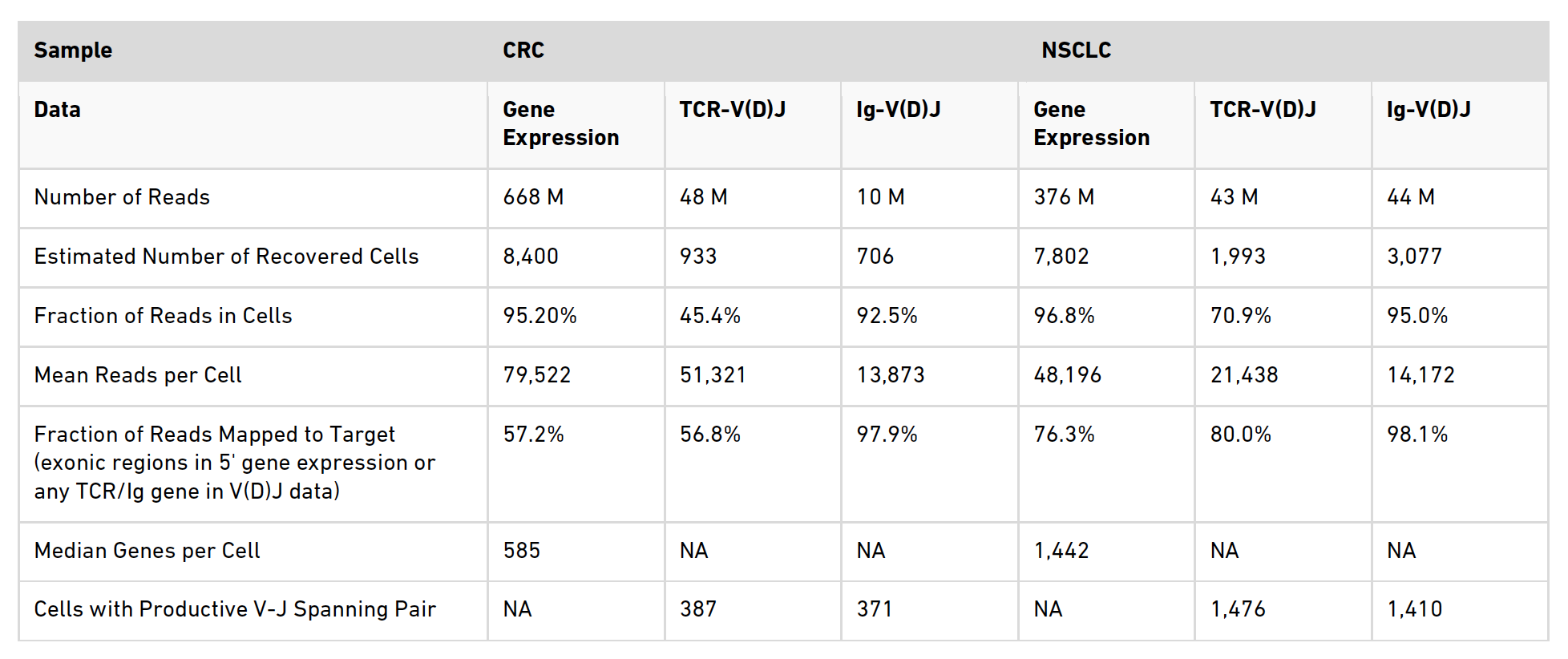
Table 1. Sequencing and performance metrics
A summary of the metrics examined in the table is provided below.
Number of reads
This is the total sequencing reads for a sample.
Estimated Number of Recovered Cells
For the gene expression data this number is total number of barcodes associated
with cell-containing partitions. Typically this is estimated from the barcode
UMI count distribution. However, there is an assumption built into the cell
calling algorithm that the RNA content between cells in a sample will only
differ by an order of magnitude (based on empirical observations). When samples
contain a highly heterogeneous mix of cells, as is the case in a tumor
environment, this assumption is not correct and consequently Cell Ranger will
under count the cells. To circumvent this you can specify the number of cells
you want Cell Ranger to call using the --force-cells option. The number chosen
to force cells to should be based on the expected cell number. However, defining
the exact number can be an iterative process and you may have to try several
different numbers of cells before getting the appropriate output. This is what
we did in both samples here, hence the reported numbers are those that were used
to force cells. For more information on the --force-cells option, see the
Cell Ranger Algorithms Overview
page. For the TCR and Ig data sets the expected number of cells is based on the
number of cells with detected immune receptor transcripts and therefore, is
expected to be lower than in the gene expression numbers as T cells and B cells
only contribute to a fraction of the total cell number.
Fraction of Reads in Cells
Is the proportion of reads that are coming from cell barcodes. Reads that are
not associated with a cell may be attributed to ambient RNA present in the
sample. You can see that for the gene expression and Ig data sets for both
samples that this metric is very high but it is lower for the TCR data sets,
suggesting some background is present in this library. For more information on
this metric see the FAQ page
How to interpret 'Fraction of Reads in Cells' metric.
Mean Reads per Cell
This is the total number of sequenced reads divided by the estimated number of
cells. Here, we targeted ~50,000 reads per cell in the gene expression data
sets, however, depending on your cell type and application it is possible to use
fewer reads than this. For more information on the number of reads per cell to
use for gene expression data, see our
Technical Note.
For the repertoire profiling (both the TCR and Ig), we targeted ~5,000 reads per
cell. You can see that we have exceeded this in some instances here, but this is
not necessary.
Fraction of Reads Mapped to Target
This is the fraction of reads that map to exons for gene expression data sets
(Reads Mapped Confidently to Exonic Regions), or to TCR/Ig sequences for the
repertoire sequencing data (Reads Mapped to Any V(D)J Gene). Here, it is good
for the NSCLC sample at around 76%, but is lower than expected in the CRC gene
expression data. This is likely due to the high proportion of dying cells in
this sample, see section 4.3 Identification of dying cells for
further information on how these cells were classified.
Median Genes per Cell
This is the median number of genes detected (with nonzero UMI counts) across all
cell-associated barcodes. This metric can provide an insight into the average
transcriptional activity of the cells in the sample.
Cells with Productive V-J Spanning Pair
This is the number of cell barcodes for which at least 1 sequence was found for
each of TRA and TRB in the case of T cells and the number of cell barcodes for
which at least 1 sequence was found for each of IGH and IGL in the case of B
cells.
To visualize the gene expression data, open Loupe Browser and import the
Loupe Browser file that you have downloaded. To open the file go to: File >
Open File. Alternatively, you can double
click on the downloaded .cloupe file to open it.
When you open the file, Loupe Browser will display the t-SNE plot generated by Cell Ranger. Each cell is represented by a dot and cells are positioned such that they are close to other cells with similar gene expression patterns. In the application note, we use the default Graph-Based clustering algorithm to identify the clusters within the t-SNE plot, but this can be changed to K-Means clustering by toggling the selection in the upper right menu bar.
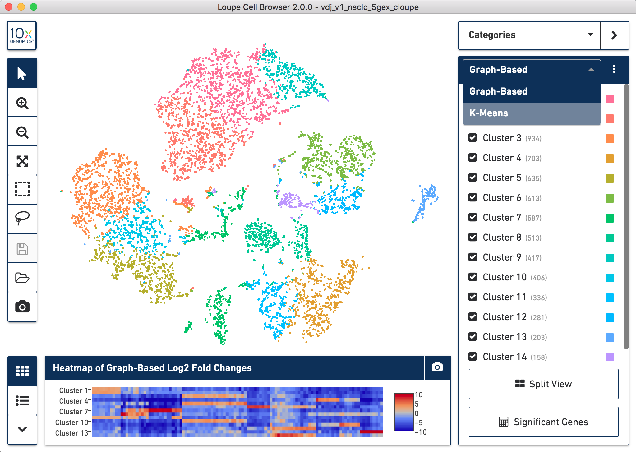
How to toggle between Graph-Based and K-Means clustering
To perform cell type classification for the different clusters, we looked at the gene expression profiles of the cells. This can be done by examining the listed upregulated genes for a specific cluster and/or by looking at the expression of known gene markers for a particular cell population. Clusters are then manually classified based on this information. Assigning cell types to clusters is an iterative process that requires looking at the gene expression patterns and coming to conclusions about the dominant cell type driving the gene expression in a particular cluster.
We show you how to do this using Loupe Browser in the video below:
Note: There will be genes you have not heard of in the gene lists for each cluster; look them up and find out what they do! Some useful websites for exploring gene functions are listed in section 7.1 Useful websites for exploring gene functions.
A common question that arises when performing cell type classification, is how do we identify dead or dying cells? In the CRC sample, we identified three clusters as dying cells (Figure 1 of the application note). When we look at the gene expression profiles of those clusters there are two things that stand out:
These two factors are indicative of poor cell health, suggesting that the cells are either about to enter or are already going through apoptosis or necrosis pathways.
In the image below you can see the gene table for cluster 3 of Graph-Based clustering in the CRC t-SNE plot (the orange cluster in the top right). In line with the criteria for identifying dead cells above, there are only 14 genes that are upregulated in this cluster and all of those that are significantly upregulated are mitochondrial genes. The expression of the genes that are upregulated in cluster 3 can also be seen in cluster 5 (the yellow/green cluster in the center), another cluster we classified as 'Dying cells'.
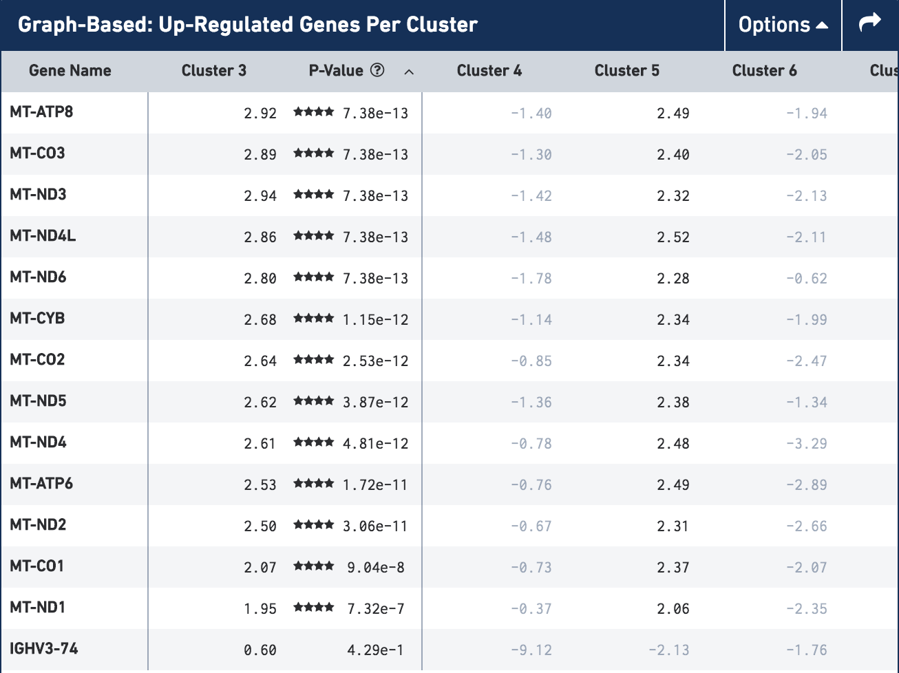
Gene table for cluster 3 (Dying cells) in the CRC t-SNE plot
To generate your figure you can export a .png of the t-SNE plot, click the
Export Plot to Image camera icon at the bottom of the left hand toolbar. Once
you have exported the image, you will need to add labels manually with the cell
type classification you have decided on.
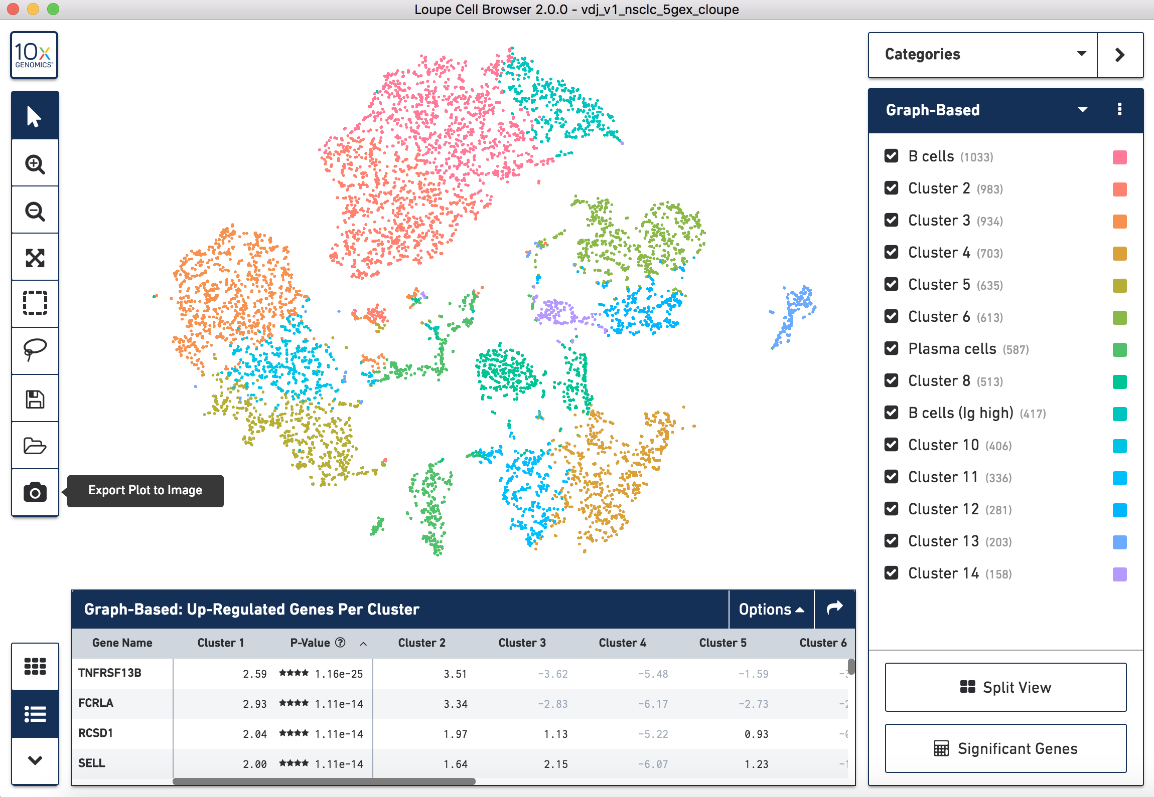
How to export a .png of the t-SNE plot for the NSCLC sample
The Single Cell Immune Profiling Solution also allows you to profile the clonotypes of the T cell receptor (TCR) and B cell immunoglobulins (Ig) from the same sample. We can examine these clonotypes in detail using Loupe V(D)J Browser. Here, we will use the corresponding TCR and Ig clonotype data from the NSCLC sample that we downloaded.
To visualize the data we can import the TCR or Ig Loupe V(D)J Browser file
into Loupe V(D)J Browser. To open the file go to: File > Open File. Alternatively,
you can double click on the downloaded .vloupe file to open it.
The landing view is a histogram of the frequency distribution of different clonotypes. These plots were used in the application note to generate Figure 2.
Looking at the clonotype distribution is only a very small part of the functionality of Loupe V(D)J Browser. For a comprehensive tutorial on how to explore your repertoire sequencing data, check out the Loupe V(D)J Browser tutorial.
To generate Figure 2, we exported the clonotype distribution plots for both TCR
and Ig data sets for our NSCLC and CRC samples. To do this, open your file of
interest, click the Export As button in the top right hand corner of the plot,
click Plot as PNG.
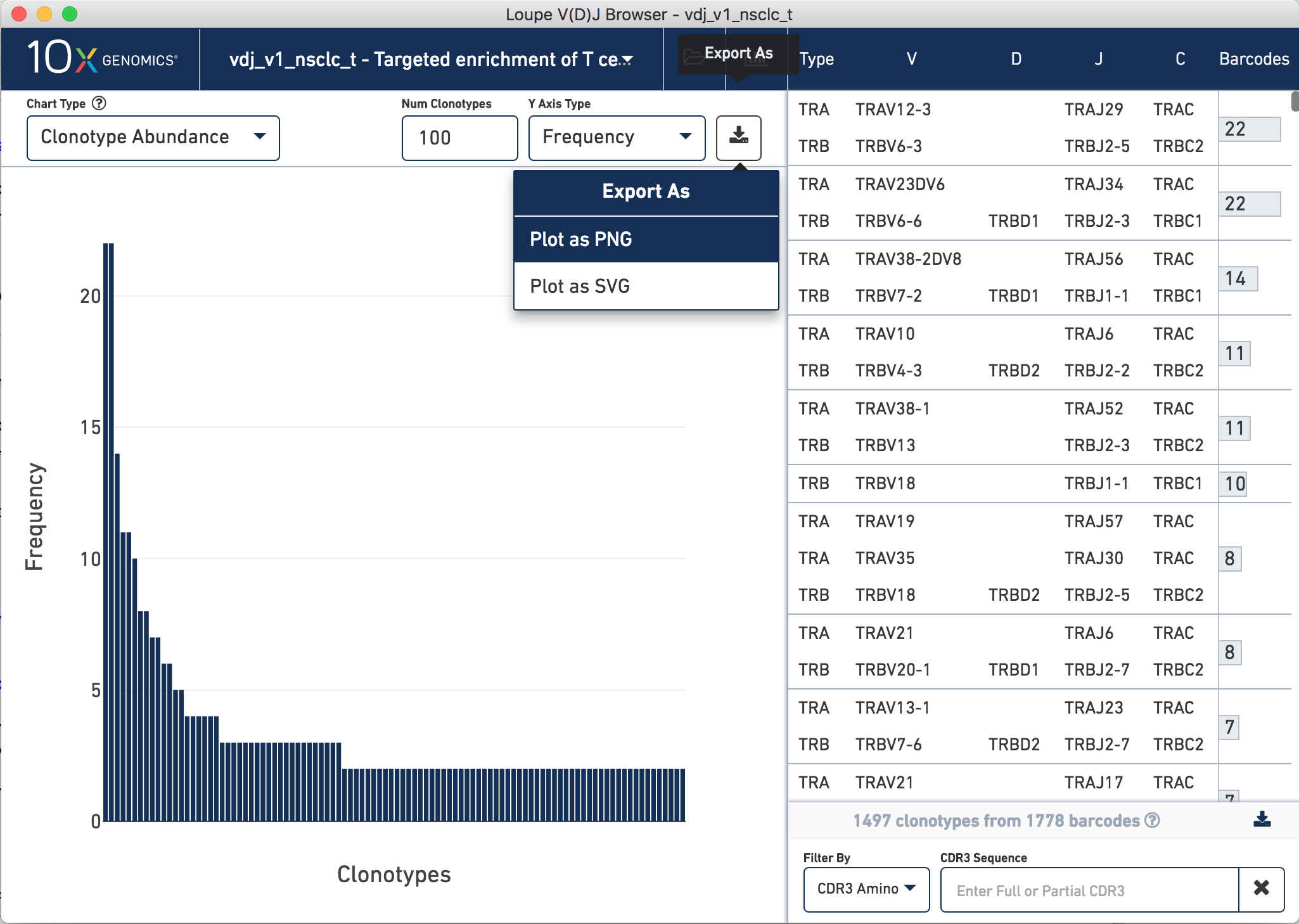
How to export a .png of the TCR clonotype frequency histogram for the NSCLC sample
One of the most powerful things about the Single Cell Immune Profiling Solution is the ability to intersect the gene expression and the repertoire sequencing data, allowing you to not only understand the cell type based on the cluster classification, but also the associated clonotype for a specific cell.
This video shows how to do this in Loupe Browser:
To generate Figure 3, we exported the image of the Ig clonotypes (light blue dots) with the dominant clone highlighted (dark blue dots), overlapped onto the t-SNE plot for the CRC sample. We then manually overlayed the annotation for the dominant clonotype onto the t-SNE plot.
In the example below we did this for the TCR clonotypes for the NSCLC sample,
but the process is the same irrelevant of sample used. Once you have loaded the
data as per the video in section 6.1, you can easily do this by clicking the
Export Plot to Image camera icon at the bottom of the left hand toolbar.
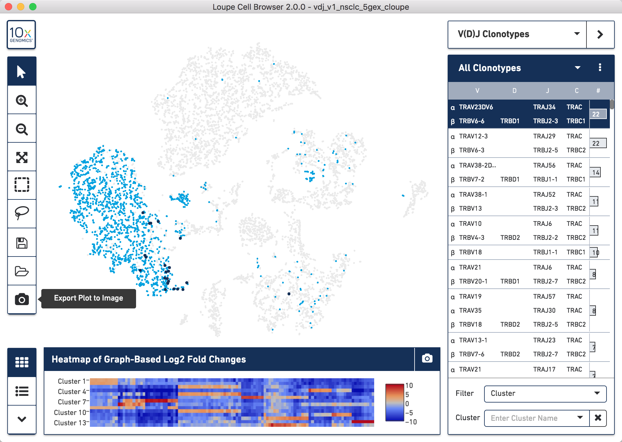
How to export a .png of the t-SNE plot with specific clonotype overlay for the NSCLC sample
www.ncbi.nlm.nih.gov/gene
www.genecards.org
www.omim.org
www.uniprot.org
www.wikipedia.org