Space Ranger6.4, printed on 03/26/2025
Goal: Evaluating image data and clustering in the spatial view.
This tutorial will showcase how to understand clusters spatially and define new clusters based on known gene markers using a preloaded mouse brain dataset in Loupe Browser.
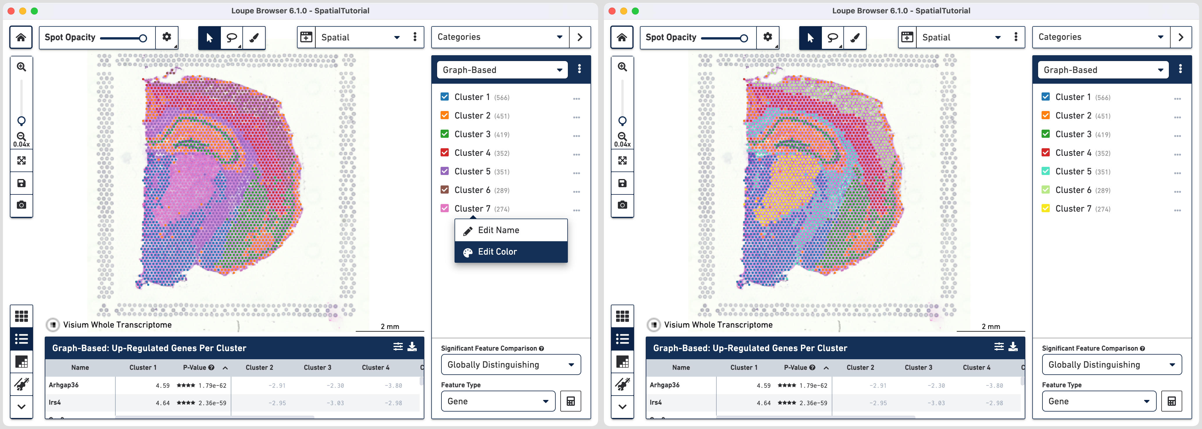
Spots that appear under the tissue are assigned to clusters by Space Ranger and are determined using only gene expression information, and without any spatial information from the image. Since each spot underneath the tissue is associated with a cluster, the clustering can be visualized in a spatial context.
First we will update the color assigned to some clusters for better distinction from tissue image. To do so, click the three horizontal dots![]() next to the cluster and select Edit Color. Here are the HEX color codes used in this tutorial:
next to the cluster and select Edit Color. Here are the HEX color codes used in this tutorial:
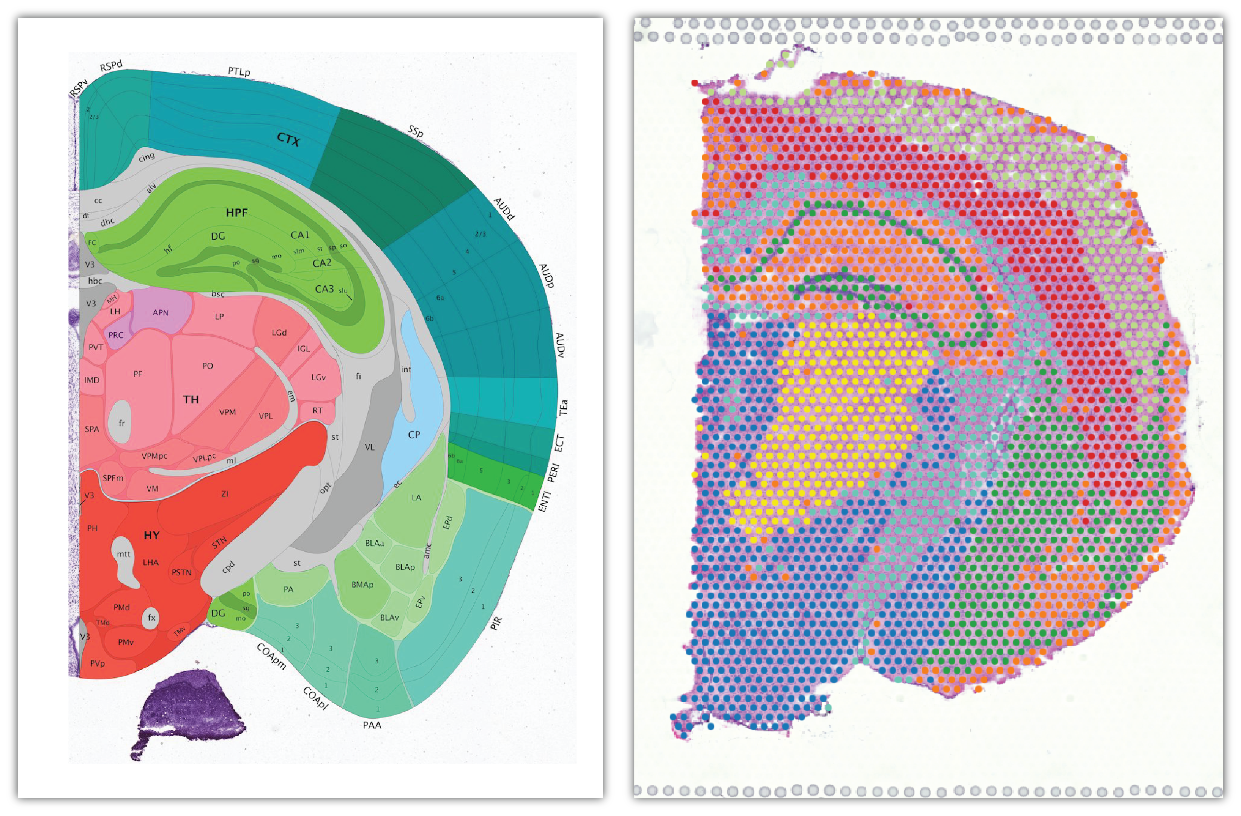
Comparing the Allen mouse brain atlas image on the left it is clear that the clustering follows the anatomical structures in the tissue.
While Loupe Browser provides visualization of clusters determined by Space Ranger, it is possible to define your own clusters based on gene markers. In this tutorial we will import a list of gene markers that correspond to subfields of hippocampus. To learn more about the use of Active Feature List refer to the Evaluate Gene Markers tutorial.
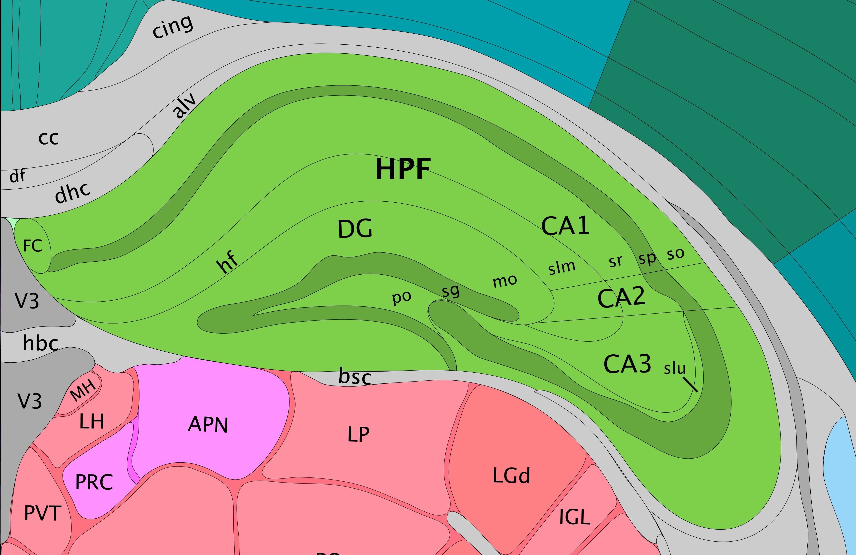
Click here to download list of genes that correspond to the CA1, CA2 and CA3 regions of the hippocampus. This file contains the following genes:
Note that the gene names must match with the ones included in the annotation reference provided to spaceranger count. See the Gene/Feature Expression mode section of the Navigation tutorial to learn more about how to construct your own lists.
To import the CSV file into Loupe Browser you will:

After it is imported, a new gene list called CA Subfields will be visible, with the three hippocampal gene markers in the list.
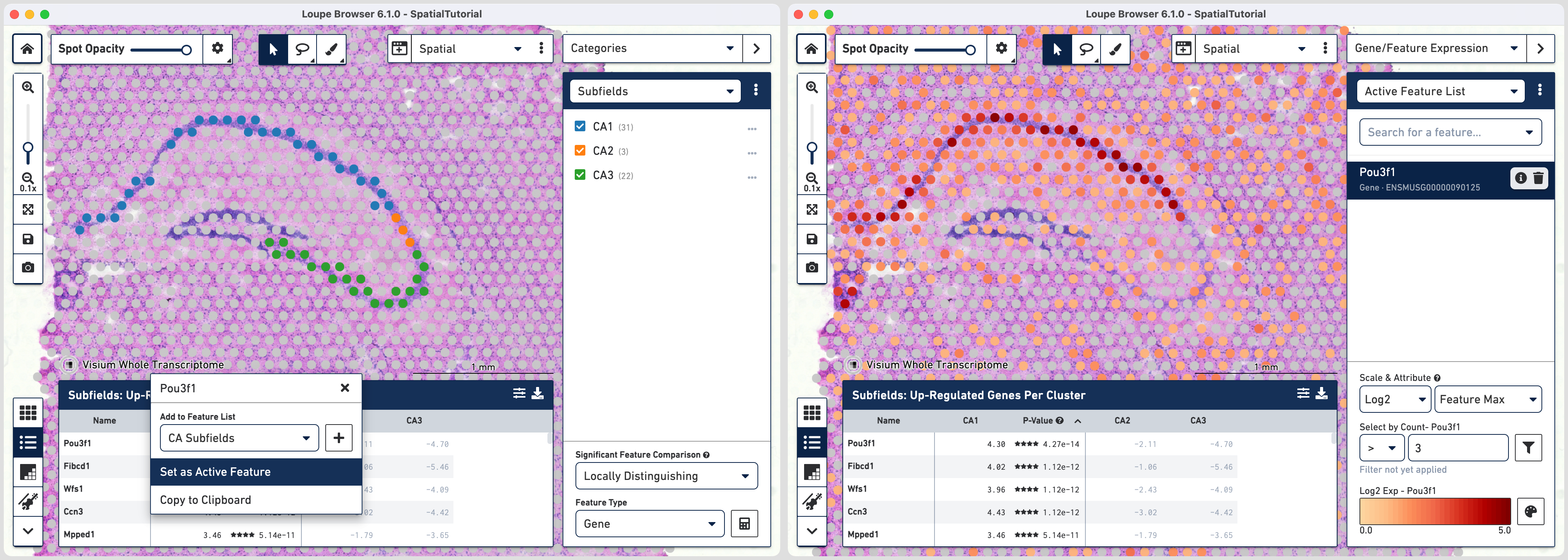
The gene Fibcd1 is a marker for CA1 subfield of the hippocampus; click on the Fibcd1 to see its expression. The dark red spots correspond to high expression for this gene. Fibcd1 is concentrated in the CA1 region and the habenula.
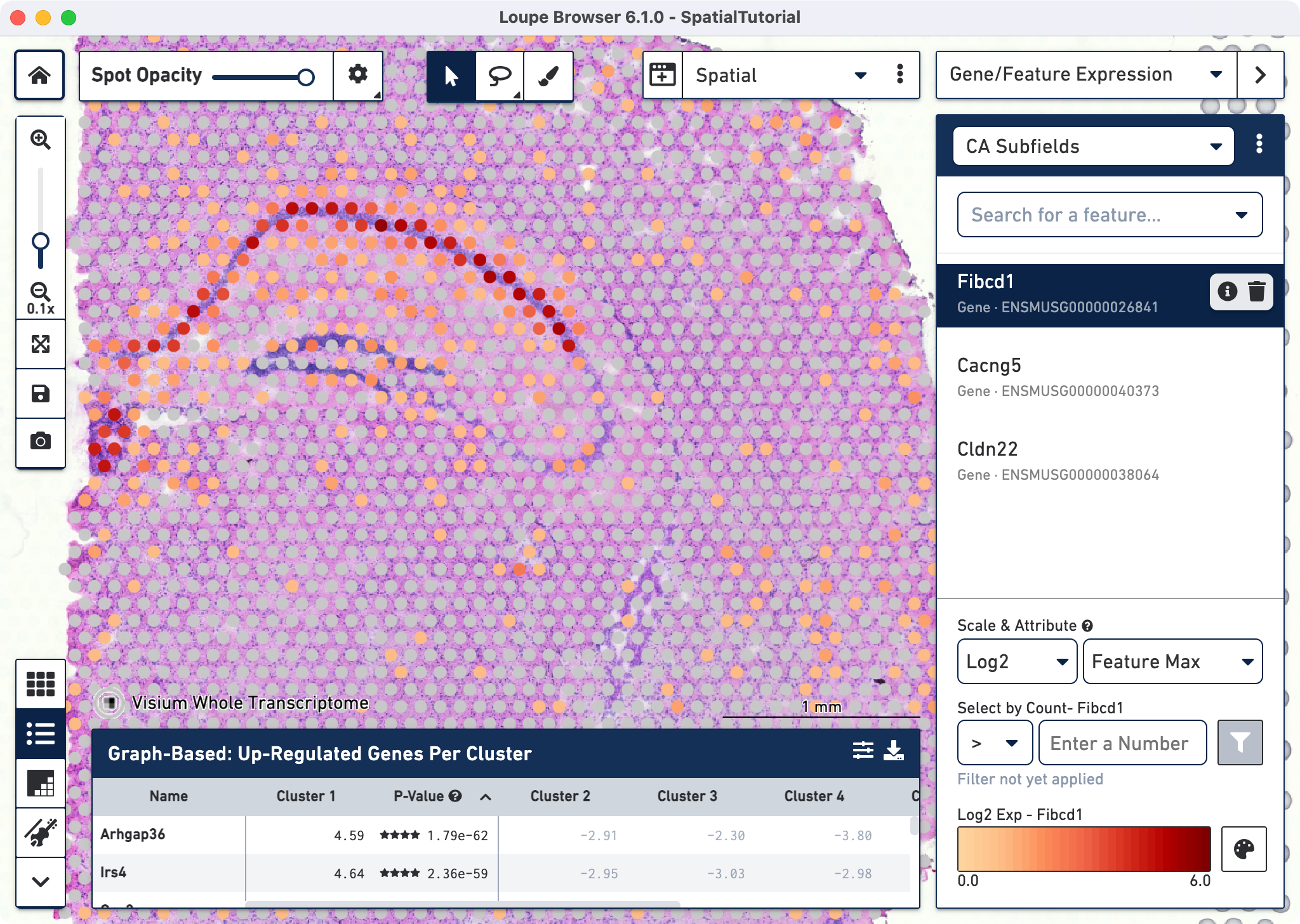
The first step to creating the CA1 cluster is to filter spots to retain only those with high expression of Fibcd1. Based on the Log2 Max Exp scale at the bottom of the Gene Expression panel, we will set a threshold of 3. This threshold was chosen as it represents the mid point in the range for log2 expression value. Enter 3 into the Select By Count field and click on the filter button![]() .
.
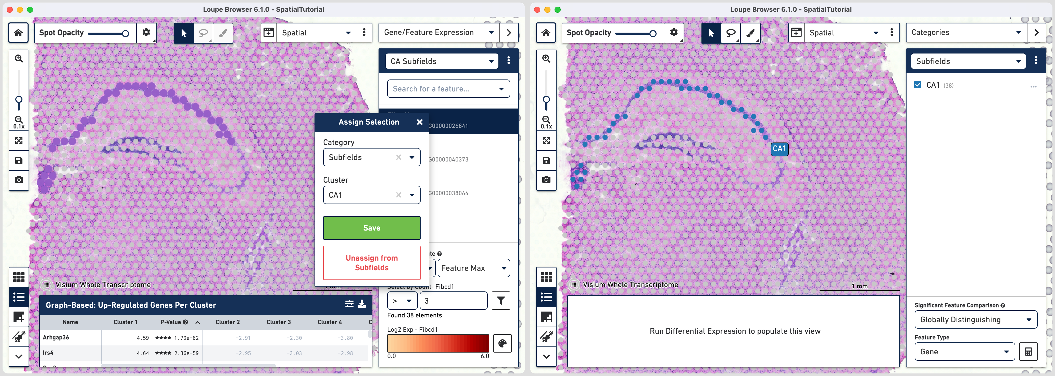
This gives us the option to create a new cluster that contains only those spots. The spots which were selected by the filter are highlighted in purple in the background. You can create a new Category name called Subfields and a new Cluster name called CA1. Once this is saved, you are taken to Category mode. The Subfields category is displayed along with the new Cluster, CA1, that we just created.
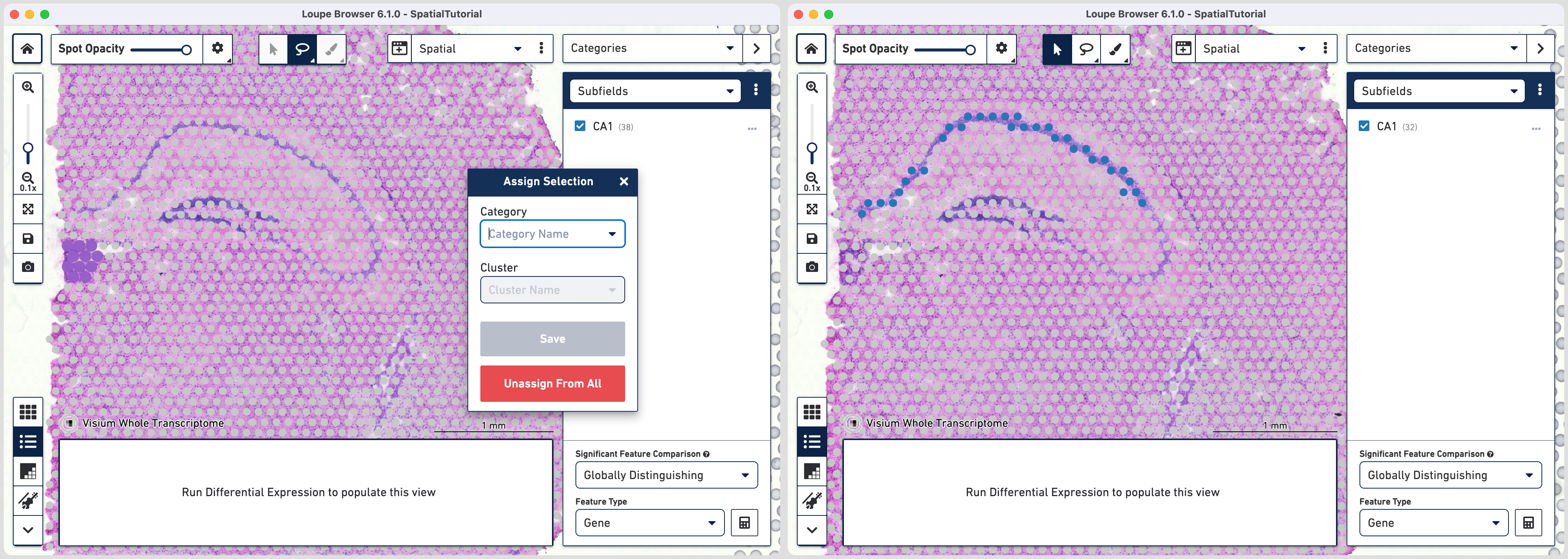
In order to isolate the CA1 region, you can remove the spots that are associated with the habenula. To do this, use the lasso tool ![]() to select the spots in the habenula and in the pop-up menu, click . The remaining spots in the cluster now correspond to only the CA1 region of the
hippocampus.
to select the spots in the habenula and in the pop-up menu, click . The remaining spots in the cluster now correspond to only the CA1 region of the
hippocampus.
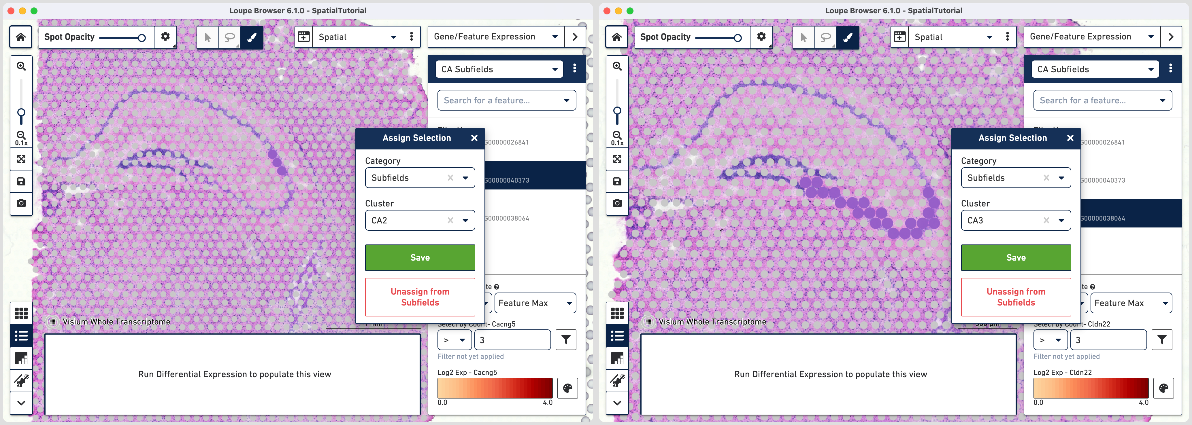
To repeat, in the mode selector, click on Gene/Feature Expression and
Since the spots associated with these genes are more spread out, it is easier to draw a outline using the brush tool ![]() and subsequently assign them to subfields.
and subsequently assign them to subfields.
Loupe Browser provides the capability to calculate new statistically significant genes for the user defined categories using two options provided at the bottom of the Categories mode. The first is Feature Type which is set to gene features for this dataset. The second is Significant Feature Comparison which offers two options in the drop down menu:
Unless the selected categories encompass the entire dataset the results for these options will vary. To learn more about the statistical methods used for calculating these results refer to the Secondary Analysis section of the algorithms page.
With the subfields defined, we can analyze the differential gene expression between these regions, choose the Locally Distinguishing option from the
Significant Feature Comparison selector in the bottom right and click calculate![]() .
.
Each subfield analysis is done comparing against the sum of the other two. For e.g. for CA1 the differential genes represent the comparison between CA1 against CA2 + CA3. After the calculations are complete, a new heatmap and data table are populated in the Data Panel on the bottom.
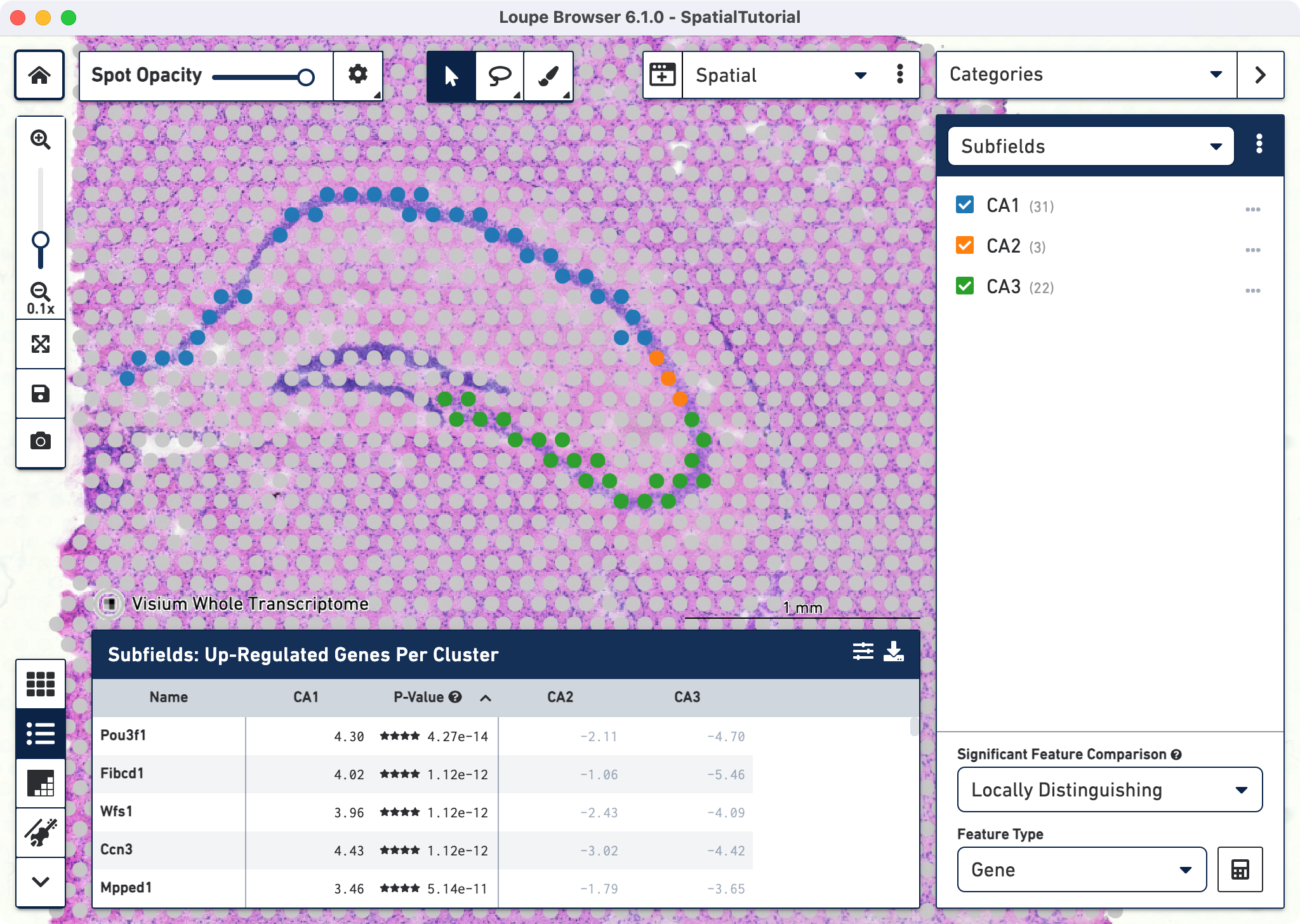
The data panel view defaults to the Feature Table ![]() . This lists the top differentially expressed up-regulated genes genes. You can change this behavior by clicking
. This lists the top differentially expressed up-regulated genes genes. You can change this behavior by clicking ![]() to change the Filter Features options. Click
to change the Filter Features options. Click ![]() to export the data table in CSV format.
to export the data table in CSV format.
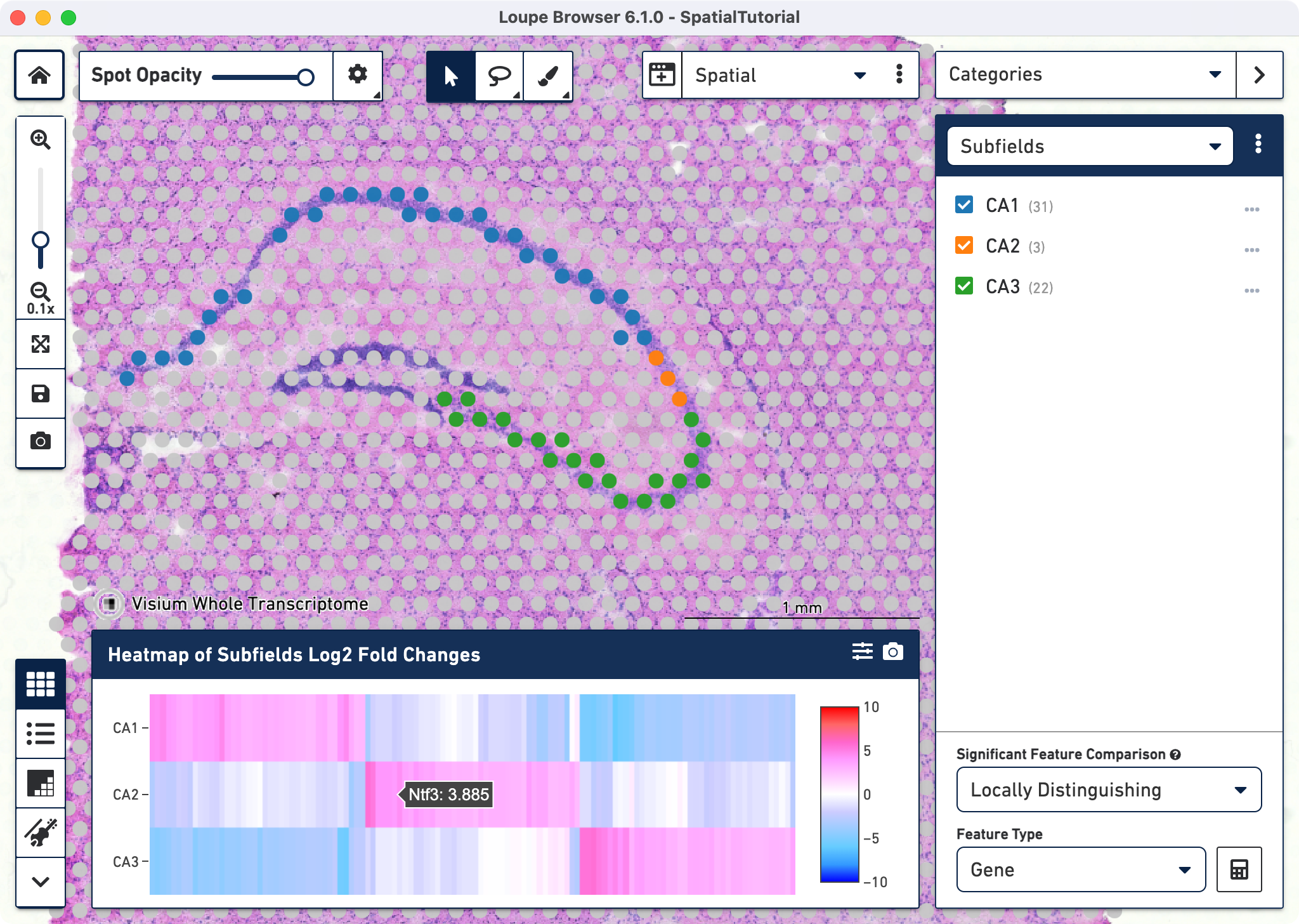
Click ![]() to access the heatmap which displays the top up-regulated genes per cluster. Each column represents the level of expression of a significant feature, and each row
represents a cluster. Grid cells are colored by a gene's log2 fold change in its cluster row, compared to the other clusters. Hovering over the columns will show the names of the features and its log2 fold change value. Click
to access the heatmap which displays the top up-regulated genes per cluster. Each column represents the level of expression of a significant feature, and each row
represents a cluster. Grid cells are colored by a gene's log2 fold change in its cluster row, compared to the other clusters. Hovering over the columns will show the names of the features and its log2 fold change value. Click ![]() to export the Heat Map in PNG format.
to export the Heat Map in PNG format.
We can now examine the region specific genes for their spatial expression patterns. Pou3f1 is a neuronal fate transcription factor that is enriched in the excitatory neurons of CA1 subfield of hippocampus. To view the resulting expression, click on the gene and select Set as Active Feature. Similarly Bok is highly enriched in CA3 and its expression pattern is consistent for the subfield.