Space Ranger6.4, printed on 04/14/2025
Goal: To evaluate the expression profiles of known gene markers of interest in the context of tissue morphology.
This tutorial will showcase how to obtain the spatial expression patterns of known gene markers associated with distinct cell types using a preloaded mouse brain dataset in Loupe Browser.
To effectively evaluate gene expression data in the context of the tissue image, it is helpful to understand the underlying morphology that can be uncovered from the tissue image. This can be achieved by making the spots transparent using the Spot Opacity slider located in the top left hand corner and moving it all the way to the left.
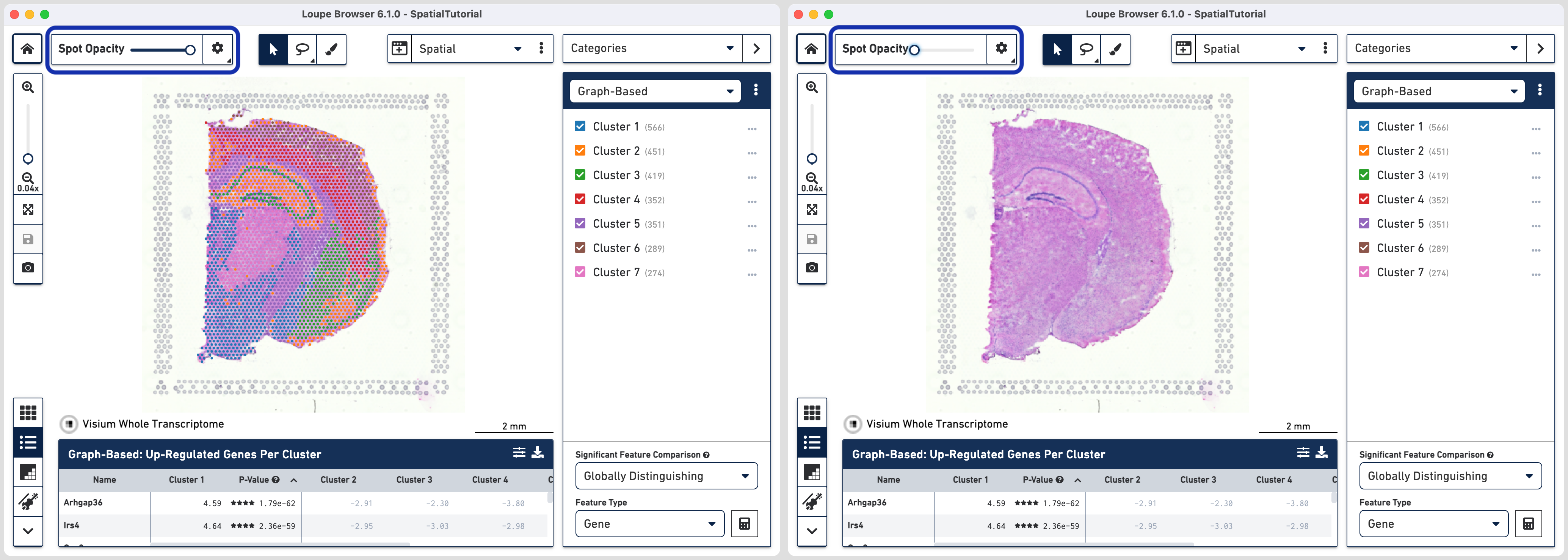
Using a combination of zoom and mouse dragging functionality navigate
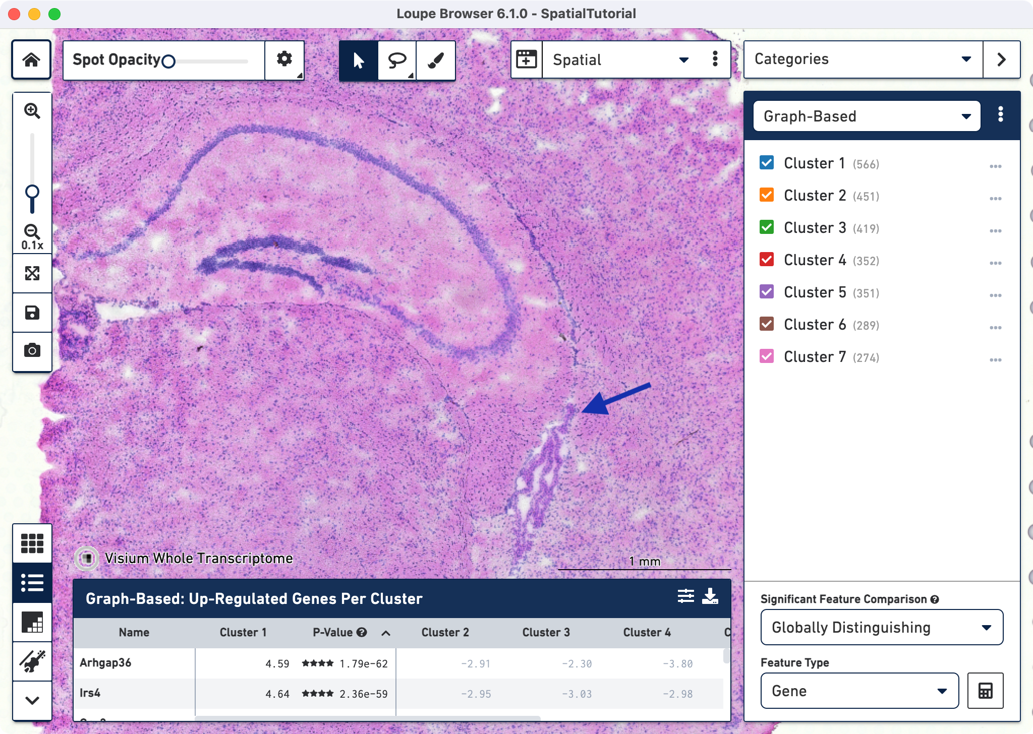
the image, evaluate the morphology, and identify landmarks of interest. You can zoom using either the mouse or the zoom slider. To revert back to default view click![]() . For
example, in this image, the curvature of the hippocampus is highlighted in blue staining. The lateral ventricle is highlighted by a blue arrow.
. For
example, in this image, the curvature of the hippocampus is highlighted in blue staining. The lateral ventricle is highlighted by a blue arrow.
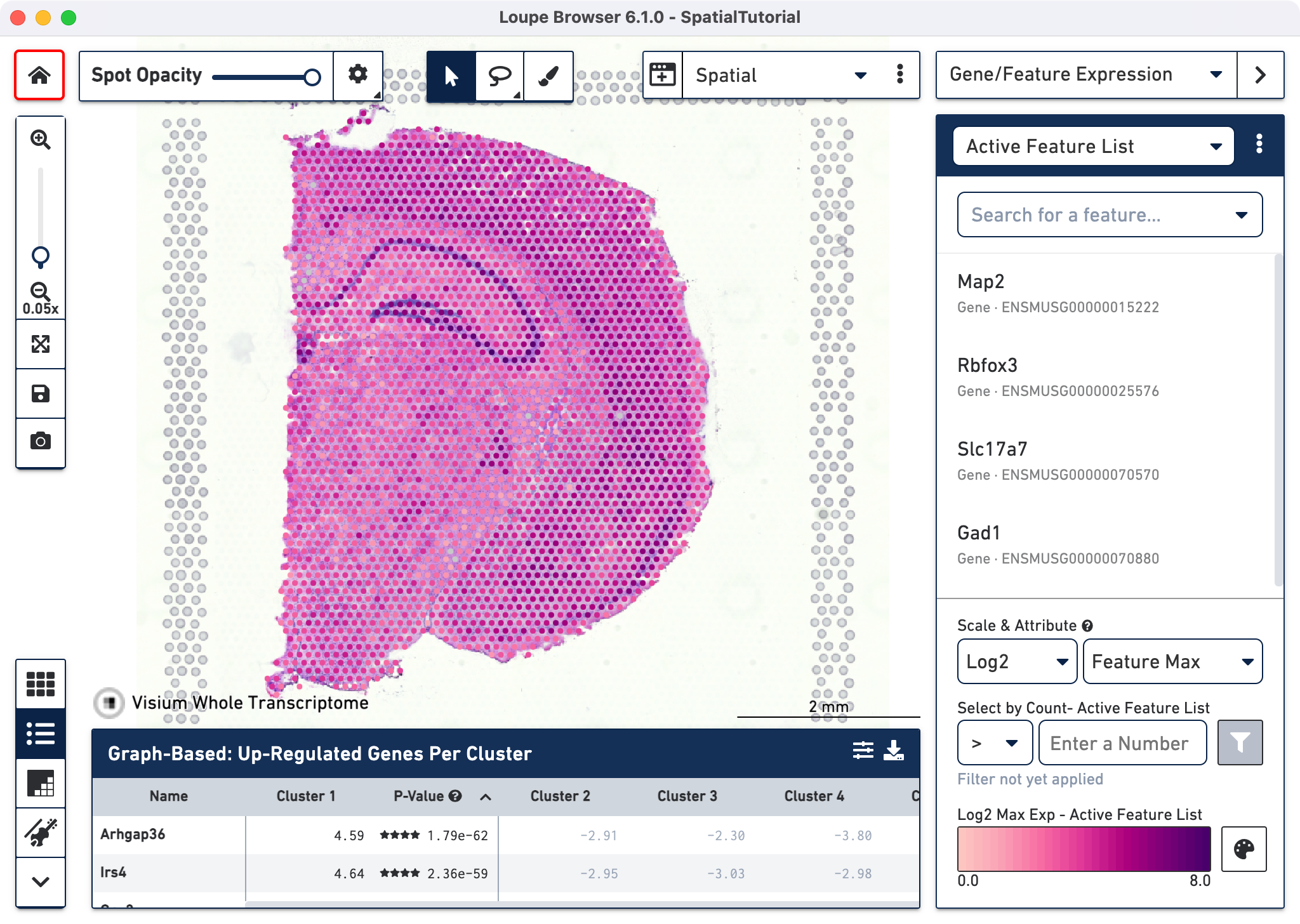
Loupe Browser provides the capability to filter the expression for specific gene or list of genes using the Active Feature List. Click on the mode selector to select Gene/Feature Expression and click on to start typing.
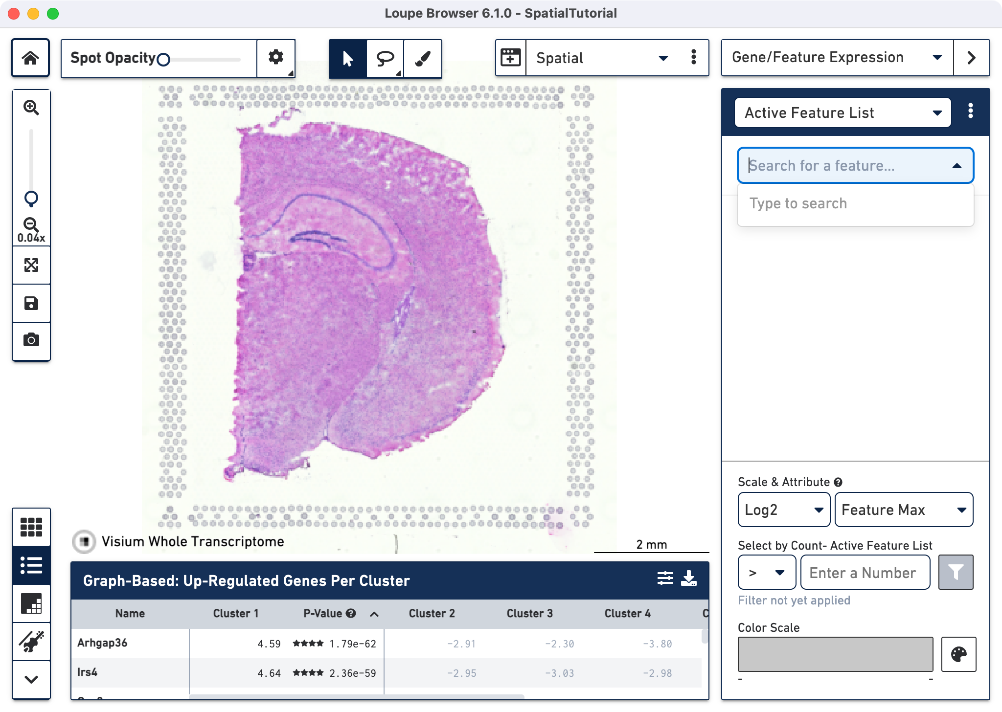
To visualize the gene expression, make the spots opaque using the Spot Opacity slider. First we will explore the neuronal cell types using some well known markers. Type Map2, which is responsible for microtubule protein that provides the structural support to neurons, in the text box. The auto-complete functionality helps to find genes of interest faster. Add the gene into the Active Feature List using any one of these methods:
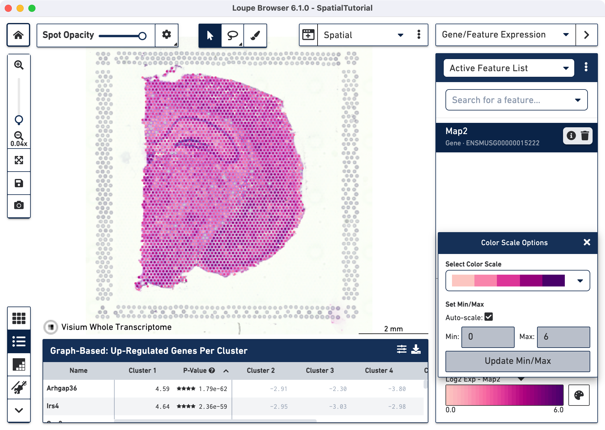
The tissue image is then updated to color-code spots based on the level of Map2 within that spot. High expression of the gene is indicated by a darker spot. As expected high Map2 expression is spread across the tissue as it is a general mature neuronal marker. Some spots appear out of the range of the color scale, in this case, light gray and correspond to spots that show no expression of the selected gene.
Hovering over a gene name reveals two icons, an information icon![]() and a trash icon
and a trash icon![]() . Clicking
. Clicking![]() loads the Ensembl reference page for that gene as a new tab in web browser. Click
loads the Ensembl reference page for that gene as a new tab in web browser. Click![]() to remove that gene from the current list. The color scale option has been updated from default using the color palette
to remove that gene from the current list. The color scale option has been updated from default using the color palette ![]() in the bottom-right corner of the browser.
in the bottom-right corner of the browser.
Next continue with these additional neuronal markers:
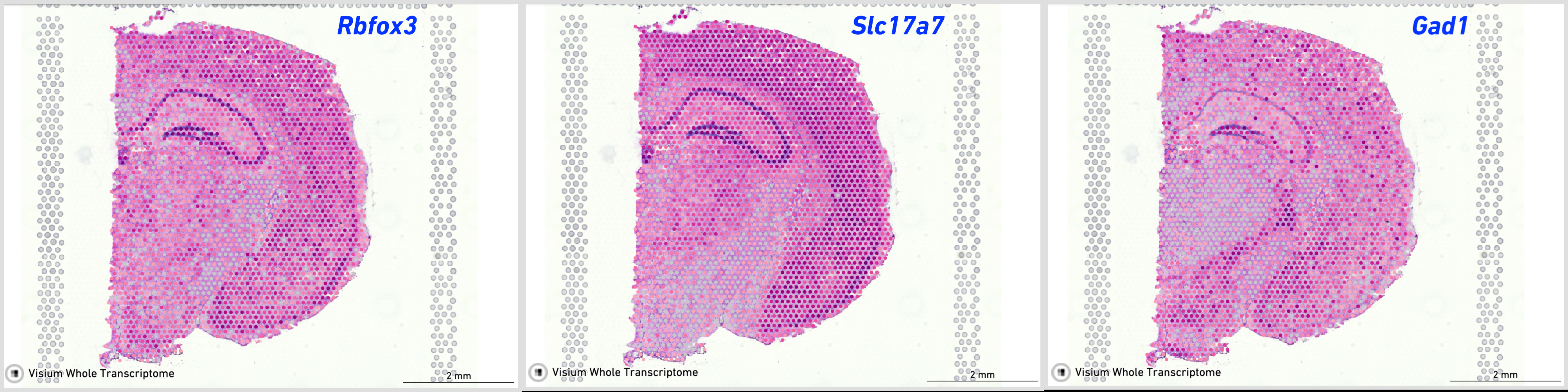
These markers give clear indication of the distinction in spatial expression. Rbfox3 and Slc17a7 are more prominently present in excitatory neurons in hippocampus and cerebral cortex while Gad1 has a heavier presence in the inhibitory neurons of the thalamus region.
Thus far, we have been examining the expression pattern for each gene. If you click the actively selected gene and deselect it, the resulting color signature represents a combination of expression levels across all the genes in the list. This allows you to visualize a set of genes associated with a cell type more confidently.
Oligodendrocytes produce myelin sheaths that surround the axons of neurons. We will use two markers to identify this cell type:
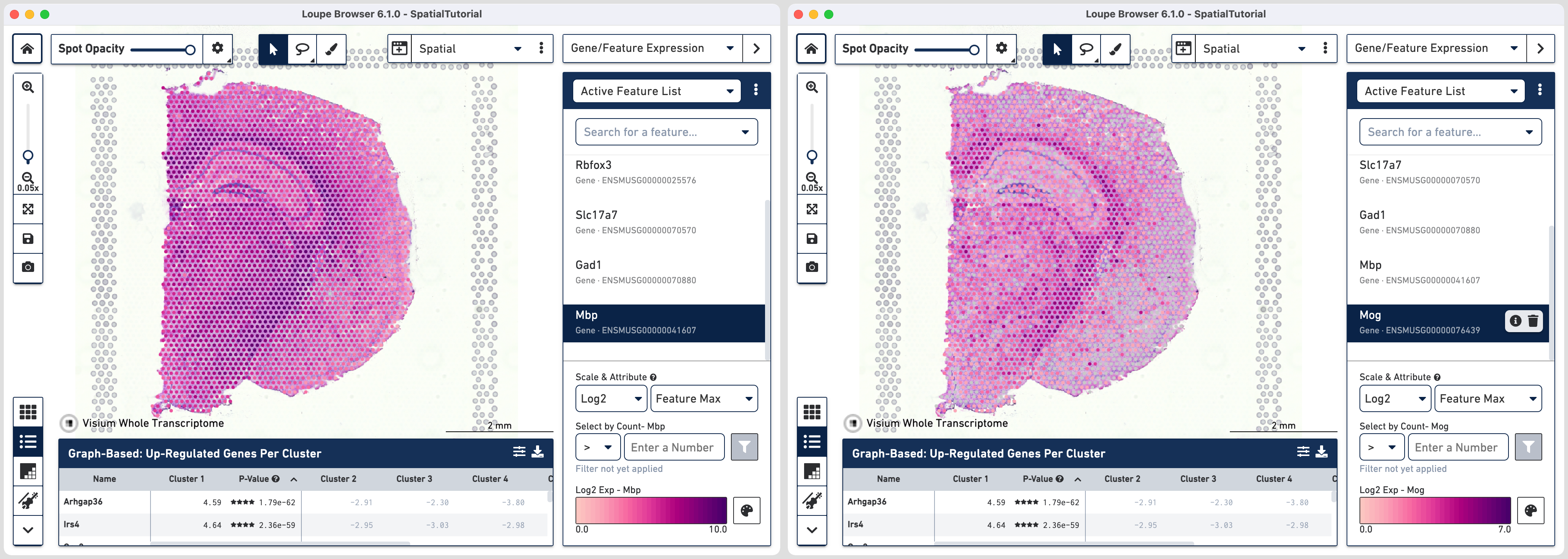
As expected the strong expression of these markers coincide with anatomical locations of the major white matter tracks including corpus callosum, fimbria, cerebral peduncle and optic track.
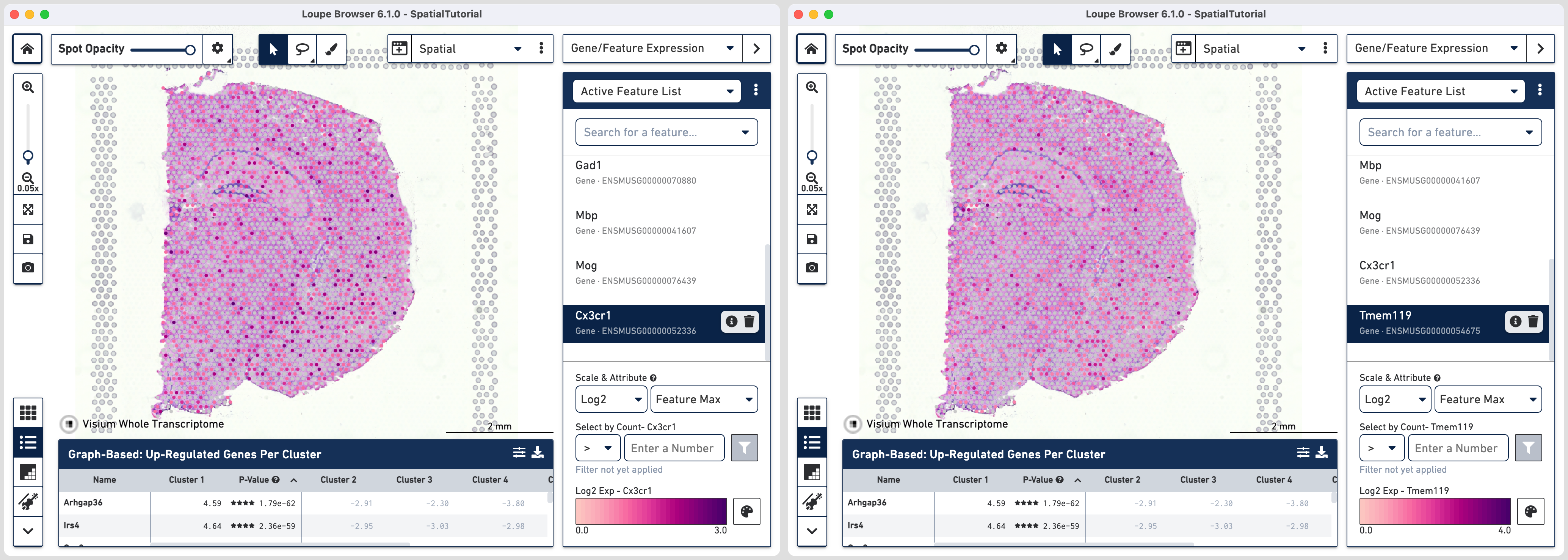
However not all genes show definite patterns in spatial expression. As an example, lets look at some markers for microglia cells which are the resident immune cells:
You can export this list for future reference by clicking the three vertical dots![]() and choosing
and choosing ![]() Export Lists option which downloads a file in CSV format to a location of your choice. The option to import a feature list is discussed in Explore Spatial Clusters tutorial.
Export Lists option which downloads a file in CSV format to a location of your choice. The option to import a feature list is discussed in Explore Spatial Clusters tutorial.
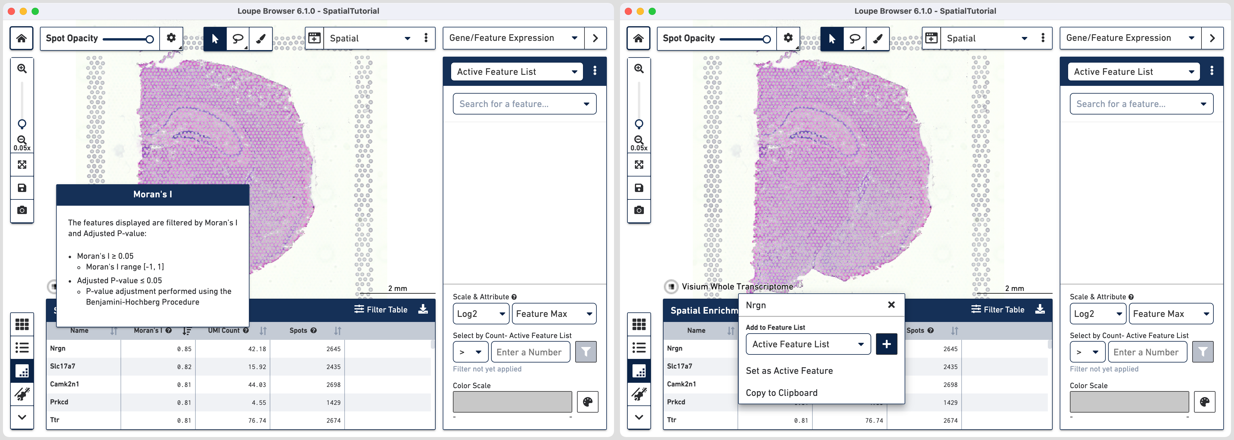
Another metric available to examine the spatial distribution of genes is by using the spatial correlation coefficient Moran's I which ranges from -1 (perfectly dispersed) to 1 (perfectly enriched). This metric is available for datasets analyzed using Space Ranger 1.3 or later.
Click on ![]() in the bottom left corner to access the spatial enrichment table. The features displayed in this table are filtered by Moran's I ≥0.05 and p-value ≤0.05 (p-value adjustment is performed using the Benjamini-Hochberg Procedure) and rounded to two decimal places to highlight the most spatially correlated features. The full list of Moran's I values for any dataset is captured in spatial_enrichment.csv which is generated in the
in the bottom left corner to access the spatial enrichment table. The features displayed in this table are filtered by Moran's I ≥0.05 and p-value ≤0.05 (p-value adjustment is performed using the Benjamini-Hochberg Procedure) and rounded to two decimal places to highlight the most spatially correlated features. The full list of Moran's I values for any dataset is captured in spatial_enrichment.csv which is generated in the outs/ folder after spaceranger count run.
The Spatial Enrichment table can be sorted by Moran's I value, UMI count, and number of Spots for which at least one valid UMI is detected for the feature. The list of features can also be filtered by a specific Moran's I value range using the Filter Table ![]() . The filtered and sorted list can be exported in CSV format by clicking
. The filtered and sorted list can be exported in CSV format by clicking![]() . Clicking on
. Clicking on ![]() next to column headers provides a pop box with information. Note that you can resize the table to display more rows using your cursor to drag the top border of the panel up. Clicking on the feature name pops a window with the option to add to Active Feature List.
next to column headers provides a pop box with information. Note that you can resize the table to display more rows using your cursor to drag the top border of the panel up. Clicking on the feature name pops a window with the option to add to Active Feature List.
We will now examine two set of genes for examples to understand spatiality. Note the values visualized correspond to the Log2 value of the Feature Max attribute.
For the first set we choose genes Ttr and Defb11. Note that you can either use the search option in the Active Feature List or click on the feature name in the spatial enrichment table to add it to the list.
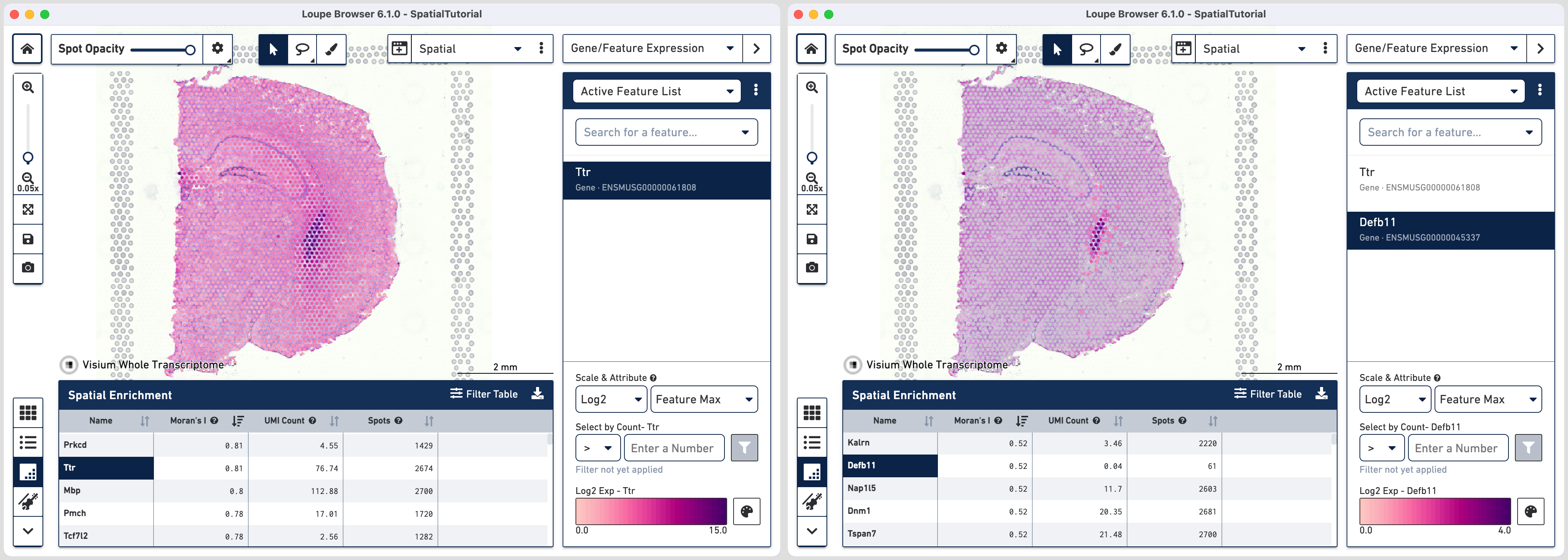
Ttr is detected across many spots (2674) and the Moran's I value is 0.81. The spatial pattern looks spread out with high expression in lateral and third ventricles. On the other hand Defb11 is detected in smaller number of spots (61), has Moran's I of 0.52 and the spatial pattern is localized to only the lateral and third ventricles. This is consistent with both the gene function and cell type association.
Ttr or Transthyretin encodes a carrier protein for thyroxine and retinol in cerebrospinal fluid (CSF) and is highly expressed in choroid plexus epithelial cells. However, it's RNA has been detected in cortex, hippocampus and thalamus. Defb11 or Defensin beta 11 encodes a antimicrobial peptide and is expressed in choroid plexus epithelial cells. Since it is in involved in innate immunity, the baseline expression in low.
For the second example, we will look at oligodendrocyte genes Mbp, Mobp and Mog.
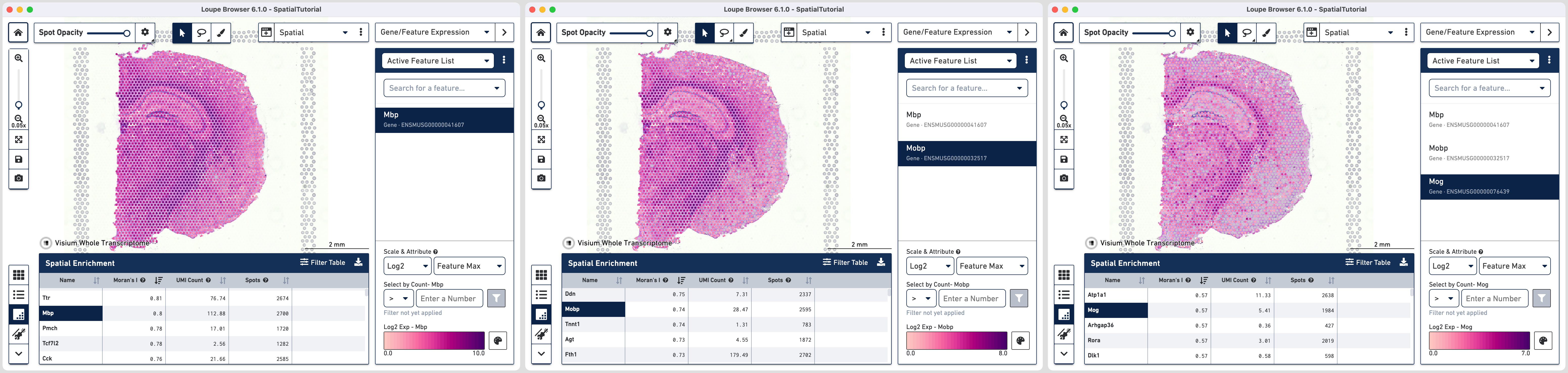
A decreasing trend of highly expressed spots is visible moving from left to right in the image above. The spatial enrichment values in the table confirm the visual observation.
| Name | Moran's I | UMI Count | Spots |
|---|---|---|---|
| Mbp | 0.8 | 112.88 | 2700 |
| Mobp | 0.74 | 28.47 | 2595 |
| Mog | 0.57 | 5.41 | 1984 |