Space Ranger2.0, printed on 03/30/2025
Many experiments involve generating data from multiple samples. Depending on the experimental design, these could be multiple Capture Areas from consecutive sections of the same tissue block, or samples from different biological conditions of the same tissue. The spaceranger aggr pipeline can be used to aggregate samples from these scenarios into a single feature-barcode matrix.
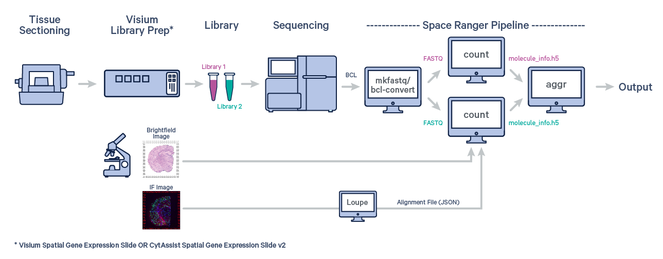
spaceranger aggr is not designed for combining multiple sequencing runs of a single capture area (e.g., resequencing the same library to increase read depth). Instead, specify all FASTQ files (--fastqs argument) in a single analysis of spaceranger count. |
The first step is to run spaceranger count on each individual capture area from the Visium slide.
For example, suppose you ran three count pipelines as follows:
$ cd /opt/runs
$ spaceranger count --id=LV123 ...
... wait for pipeline to finish ...
$ spaceranger count --id=LB456 ...
... wait for pipeline to finish ...
$ spaceranger count --id=LP789 ...
... wait for pipeline to finish ...
Now you can aggregate these three runs to get a single feature-barcode matrix and analysis. In order to do so, you need to create an aggregation CSV.
Create a CSV file with a header line containing the following columns:
| Column Name | Description |
|---|---|
library_id | Required. Unique identifier for this input capture area. This will be used for labeling purposes only; it doesn't need to match any previous ID you have assigned to the capture area. |
molecule_h5 | Required. Path to the molecule_info.h5 file produced by spaceranger count. For example, if you processed your capture area by calling spaceranger count --id=ID in some directory /DIR, this path would be /DIR/ID/outs/molecule_info.h5. |
cloupe_file | Required. Path to the cloupe.cloupe file produced by spaceranger count. For example, if you processed your capture area by calling spaceranger count --id=ID in some directory /DIR, this path would be /DIR/ID/outs/cloupe.cloupe. |
spatial_folder | Optional. Path to the spatial folder produced by spaceranger count. For example, if you processed your capture area by calling spaceranger count --id=ID in some directory /DIR, this path would be /DIR/ID/outs/spatial.Note that not specifying the spatial_folder column will lead to the aggregated tissue positions list (aggr_tissue_positions.csv) and spatial folder containing spatial images and scalefactors (spatial/) to be omitted from the outs/ folder generated from the spaceranger aggr run. |
You can either make the CSV file in a text editor, or create it in Excel and export to CSV. Continuing the example from the previous section, your Excel spreadsheet would look like this:
| A | B | C | D (optional) | |
|---|---|---|---|---|
| 1 | library_id | molecule_h5 | cloupe_file | spatial_folder |
| 2 | LV123 | /opt/runs/LV123/outs/molecule_info.h5 | /opt/runs/LV123/outs/cloupe.cloupe | /opt/runs/LV123/outs/spatial |
| 3 | LB456 | /opt/runs/LB456/outs/molecule_info.h5 | /opt/runs/LB456/outs/cloupe.cloupe | /opt/runs/LB456/outs/spatial |
| 4 | LP789 | /opt/runs/LP789/outs/molecule_info.h5 | /opt/runs/LP789/outs/cloupe.cloupe | /opt/runs/LP789/outs/spatial |
When you save it as a CSV, the result would look like this:
library_id,molecule_h5,cloupe_file,spatial_folder
LV123,/opt/runs/LV123/outs/molecule_info.h5,/opt/runs/LV123/outs/cloupe.cloupe,/opt/runs/LV123/outs/spatial
LB456,/opt/runs/LB456/outs/molecule_info.h5,/opt/runs/LB456/outs/cloupe.cloupe,/opt/runs/LB456/outs/spatial
LP789,/opt/runs/LP789/outs/molecule_info.h5,/opt/runs/LP789/outs/cloupe.cloupe,/opt/runs/LP789/outs/spatial
In addition to the CSV columns expected by spaceranger aggr, you may optionally supply additional columns containing library meta-data (e.g., lab or sample origin). These custom library annotations do not affect the analysis pipeline but can be visualized downstream in the Loupe Browser (see below). Note that unlike other CSV inputs to Spaceranger, these custom columns may contain characters outside the ASCII range (e.g., non-Latin characters).
It is possible to assign categories and values to individual samples prior to the spaceranger aggr run by adding additional columns to the aggregation CSV. These category assignments propagate into Loupe Browser, where you can view them, and determine genes that drive differences between samples. For example, the following spreadsheet was used to aggregate the tutorial dataset:
| A | B | C | D | |
|---|---|---|---|---|
| 1 | library_id | molecule_h5 | cloupe_file | AMLStatus |
| 2 | AMLNormal1 | /path/to/AMLNormal1/outs/molecule_info.h5 | /path/to/AMLNormal1/outs/cloupe.cloupe | Normal |
| 3 | AMLNormal2 | /path/to/AMLNormal2/outs/molecule_info.h5 | /path/to/AMLNormal2/outs/cloupe.cloupe | Normal |
| 4 | AMLPatient | /path/to/AMLPatient/outs/molecule_info.h5 | /path/to/AMLPatient/outs/cloupe.cloupe | Patient |
Any columns in addition to library_id, molecule_h5, cloupe_file and spatial_folder will be converted into
categories, and the spots in each sample will be assigned to one of the values
in that category.
spaceranger aggr does not perform batch correction for removal of technical artifacts due to differences in assays. For this reason, 10x Genomics does not recommend combining Visium data from fundamentally different treatments such as different staining protocols (e.g. immunofluorescence vs H&E stained tissue sections), different tissue storage conditions (e.g. Fresh Frozen vs FFPE tissue sections), different library preparation protocols (e.g. short cDNA vs long cDNA), or other variations in the assay preparation.
These are the most common command line arguments (run spaceranger aggr --help for a full list):
| Argument | Description |
|---|---|
--id=ID | Required. A unique run ID string: e.g. AGG123 |
--csv=CSV | Required. Path to the aggregation CSV file containing a list of spaceranger count outputs (see Setting up a CSV). |
--normalize=MODE | Optional. String specifying how to normalize depth across the input libraries. Valid values: mapped (default), or none (see Depth Normalization). |
After specifying these input arguments, run spaceranger aggr:
$ cd /opt/runs
$ spaceranger aggr --id=AGG123 \
                  --csv=AGG123_libraries.csv \
                  --normalize=mapped
The pipeline will begin to run, creating a new folder named with the aggregation ID you specified (e.g. /opt/runs/AGG123) for its output. If this folder already exists, spaceranger will assume it is an existing pipestance and attempt to resume running it.
The spaceranger aggr pipeline generates output files that contain all of the data from the individual input jobs, aggregated into single output files, for convenient multi-sample analysis. Refer to the Understanding Outputs section to learn about aggr output files.
When combining multiple capture areas, the barcode sequences for each channel are distinguished by a capture area suffix appended to the barcode sequence (see Capture Area).
By default, the reads from each capture area are subsampled such that all capture areas have the same effective sequencing depth, measured in terms of reads that are confidently mapped to the transcriptome or assigned to the feature IDs per spot. However, it is possible to change the depth normalization mode (see Depth Normalization).
New slide versions and chemistries were introduced in Space Ranger 2.0. Aggregating samples must obey the chemistry compatibility matrix. Data from Visium for FFPE sections is supported by spaceranger aggr provided that the same probe set reference CSV file (#) is used for all samples.
| The slide combinations aggregated with spaceranger aggr are either supported (validated by 10x), or unsupported. Samples run on the same slide version can be aggregated, except those with slide serial numbers starting with V1 or V2. |
| Visium Spatial Gene Expression | Visium Spatial Targeted | Visium Spatial Gene Expression for FFPE | CytAssist Spatial Gene Expression for FFPE | |
|---|---|---|---|---|
| Command line option | --target-panel |
--probe-set |
--cytaimage & --probe-set |
|
| Visium Spatial Gene Expression | Supported | Supported | Unsupported | Unsupported |
| Visium Spatial Targeted | Supported | Unsupported | Unsupported | |
| Visium Spatial Gene Expression for FFPE | Supported# | Unsupported | ||
| CytAssist Spatial Gene Expression for FFPE | Supported# |
The spaceranger aggr command can aggregate results that include Targeted Spatial Gene Expression analyses, provided that the same target panel CSV file is used for the targeted libraries, and can also be aggregated with whole transcriptome Spatial Gene Expression libraries. Secondary analysis for all libraries is done with the non-targeted genes excluded from the feature-barcode matrices. Aggregated feature-barcode matrices follow the same convention as Targeted Spatial Gene Expression analysis: the filtered feature-barcode matrices do not include non-targeted genes, whereas the raw feature-barcode matrices include all genes.
When combining data from multiple capture areas, the spaceranger aggr pipeline automatically equalizes the read depth between groups before merging, which is the recommended approach in order to avoid the batch effect introduced by sequencing depth. It is Possible to turn off normalization or change the way normalization is done. The none option may be appropriate if you want to maximize sensitivity and plan to deal with depth normalization in a downstream step.
There are two normalization modes:
| Argument | Description |
|---|---|
--normalize=mapped | Default. Subsample reads from higher-depth capture areas until they all have, on average, an equal number of reads per tissue covered spot that are confidently mapped to the transcriptome. If Targeted Spatial Gene Expression libraries are included, then normalization is performed on the basis of mean reads per spot mapped confidently to the targeted transcriptome. The subsampling rates for Targeted Spatial Gene Expression libraries are multiplied by 2, provided all libraries can achieve that depth. This multiple is consistent with sequencing depth recommendations and is also done to avoid removing large fractions of reads from targeted libraries whenever they are combined with whole transcriptome libraries. |
--normalize=none | Optional. Do not normalize at all. |
Each capture area is a physically distinct partition on a Visium slide. However, each of these capture areas are printed with the same set of barcode tagged mRNA capture sequences known as the barcode whitelist. To keep the barcodes unique when aggregating multiple libraries, we append a small integer identifying the capture area to the barcode nucleotide sequence, and use that nucleotide sequence plus ID as the unique identifier in the feature-barcode matrix. For example, AAACAACGAATAGTTC-1 and AAACAACGAATAGTTC-2 are distinct spot barcodes from different capture areas, despite having the same barcode nucleotide sequence.
This number, called the capture area suffix, tells us which capture area the barcode sequence came from. The numbering of the capture area will reflect the order that the capture area were provided in the Aggregation CSV.