Cell Ranger6.4, printed on 03/29/2025
This tutorial demonstrates the basic workflow for Single Cell Gene Expression data analysis with Loupe Browser, including quality control (QC), clustering, cell annotation, cell abundance analysis, and differential gene expression. The tutorial uses 5’ Single Cell Gene Expression data, however, all the steps also apply to 3' Single Cell Gene Expression data.
| This tutorial was run with Cell Ranger v7.0 and Loupe Browser v6.2.0. We recommend completing the Filtering and Reclustering Workflow tutorial first. |
The 5' Single Cell Gene Expression datasets (v2) used in this tutorial were obtained from the Asian Immune Diversity Atlas (AIDA) project. These eight datasets represent four samples (JP_RIK_H040, JP_RIK_H041, KR_SGI_H128, and KR_SGI_H131) from two healthy Japanese donors and two healthy South Korean donors (each sample has two libraries):
1. JP_RIK_B003_L001_5GEX_H040 (Japan_RIKEN_Batch3_Library1_HealthyDonor040)
2. JP_RIK_B003_L002_5GEX_H040 (Japan_RIKEN_Batch3_Library2_HealthyDonor040)
3. JP_RIK_B003_L001_5GEX_H041 (Japan_RIKEN_Batch3_Library1_HealthyDonor041)
4. JP_RIK_B003_L002_5GEX_H041 (Japan_RIKEN_Batch3_Library2_HealthyDonor041)
5. KR_SGI_B010_L001_5GEX_H128 (S.Korea_SGI_Batch10_Library1_HealthyDonor128)
6. KR_SGI_B010_L002_5GEX_H128 (S.Korea_SGI_Batch10_Library2_HealthyDonor128)
7. KR_SGI_B010_L001_5GEX_H131 (S.Korea_SGI_Batch10_Library1_HealthyDonor131)
8. KR_SGI_B010_L002_5GEX_H131 (S.Korea_SGI_Batch10_Library2_HealthyDonor131)
The raw FASTQ files were analyzed with the cellranger count pipeline, followed by cellranger aggr. The steps in this tutorial are performed in Loupe Browser, after loading the cloupe.cloupe output file from cellranger aggr (see appendix for the cellranger commands).
Download these files to follow along with the tutorial:
First, use the filtering and reclustering workflow in Loupe Browser to perform quality control (QC) based on three metrics: 1) UMI counts, 2) the number of detected genes, and 3) the percentage of mitochondrial genes.
After opening the tutorial .cloupe file, click the Recluster button in the Categories Mode panel:
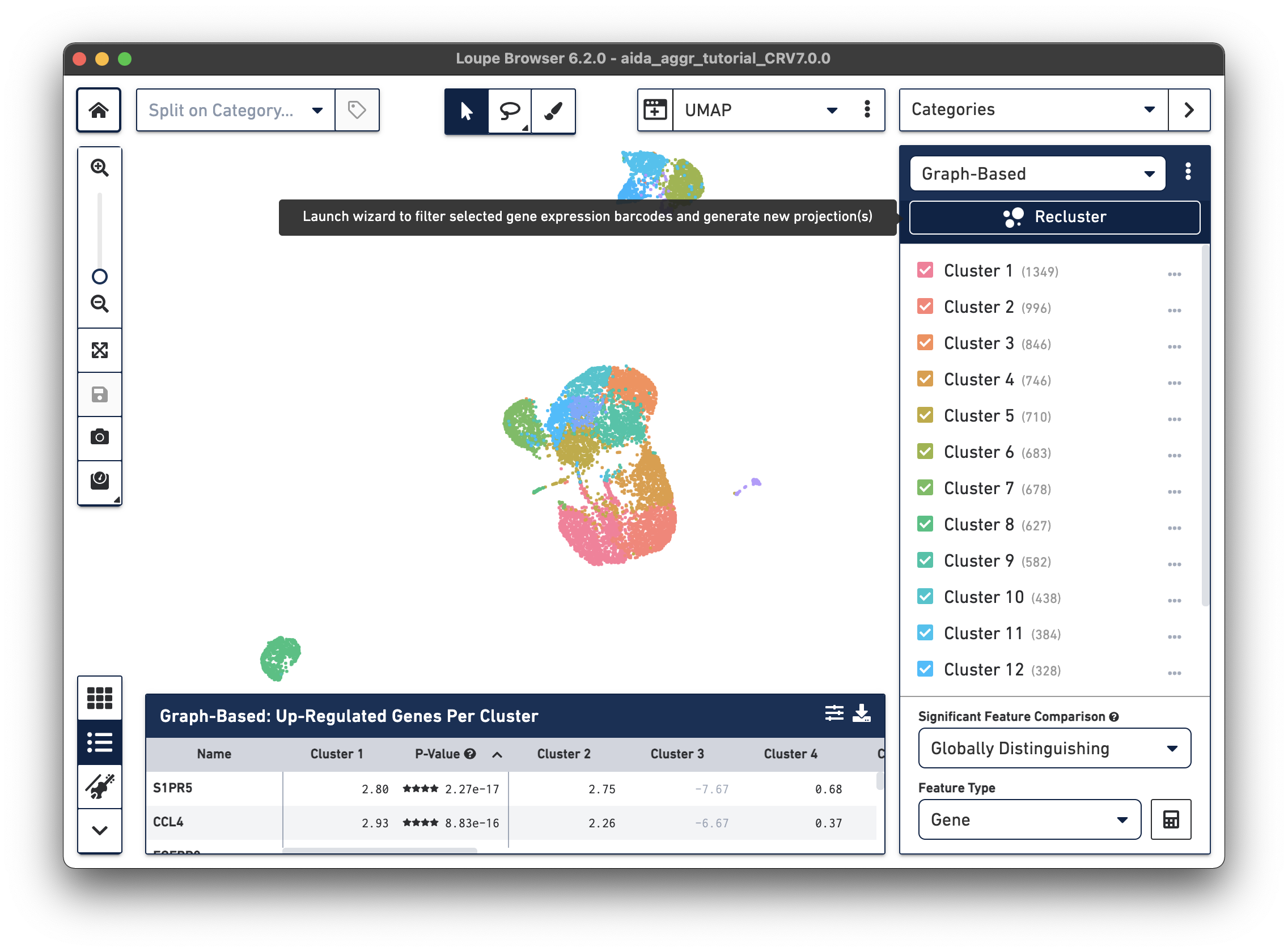
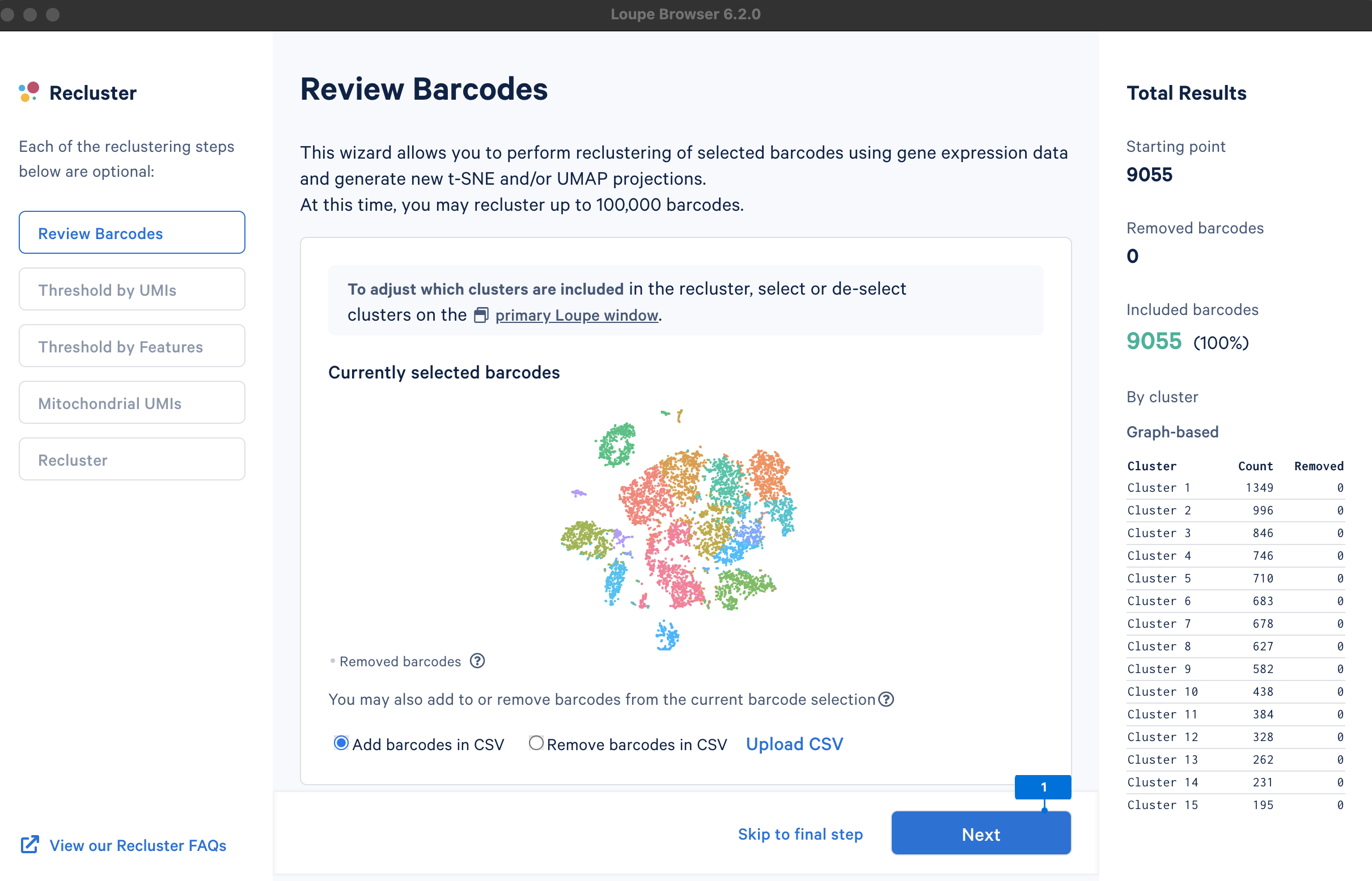
A new window will open with the Recluster module.
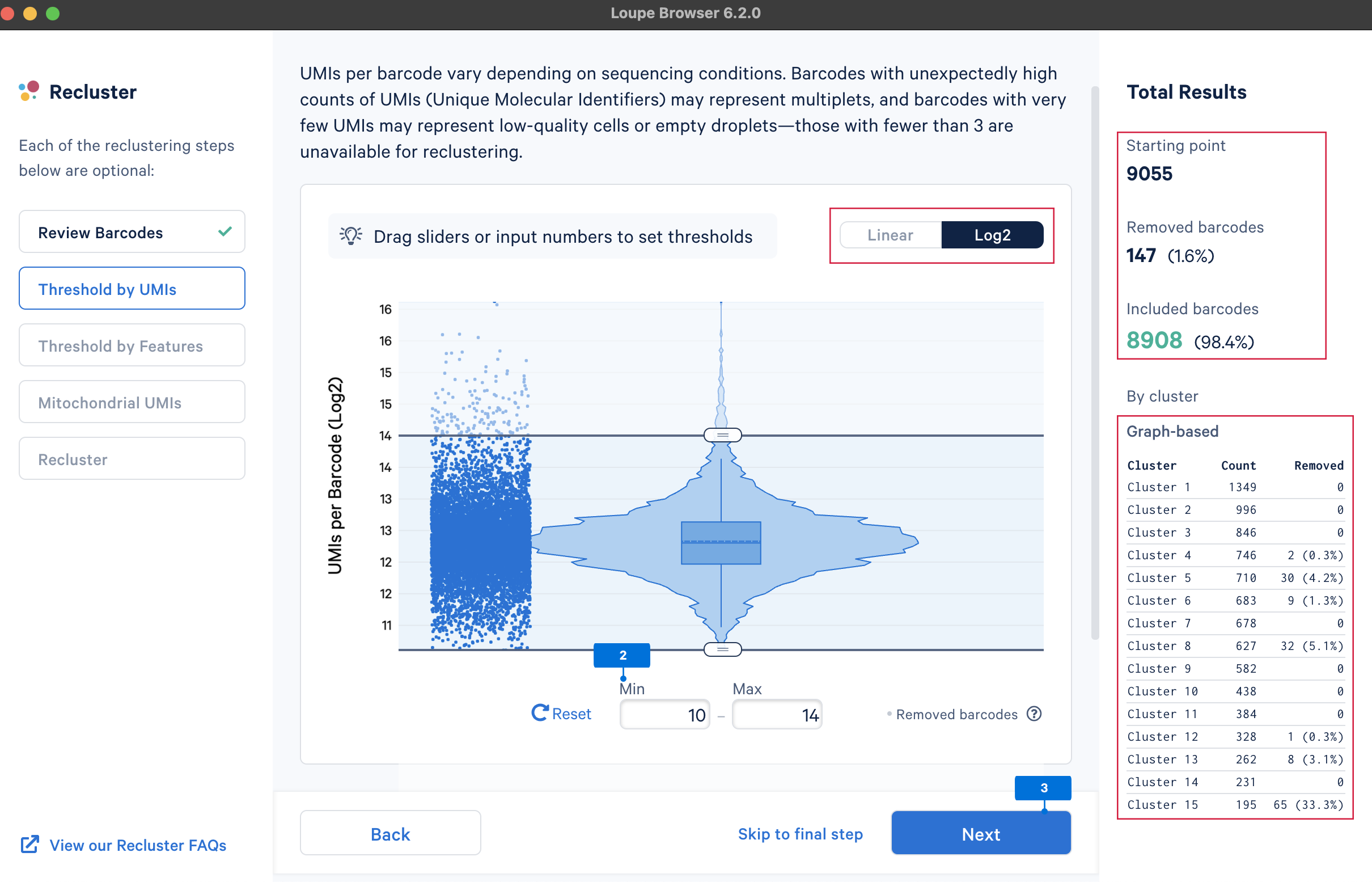
The main goal of this step is to remove outliers, which could potentially be low-quality cells (very low UMI counts) or doublets (very high UMI counts). There are no universal criteria to filter UMI counts since different sample and cell types have distinct UMI levels (e.g., tumor samples may have higher RNA content compared to PBMCs; in PBMC samples, some disease states may result in greater abundance of higher RNA content plasma B cells or lower RNA content platelets (see Yamawaki et al. 2021)). Selection of the UMI range should be based on biological knowledge about the sample and may be an iterative process. UMI counts can be visualized on the linear or log2 scale.
We will select the barcodes containing UMI counts between 210 and 214 (most of the cells are within this range).
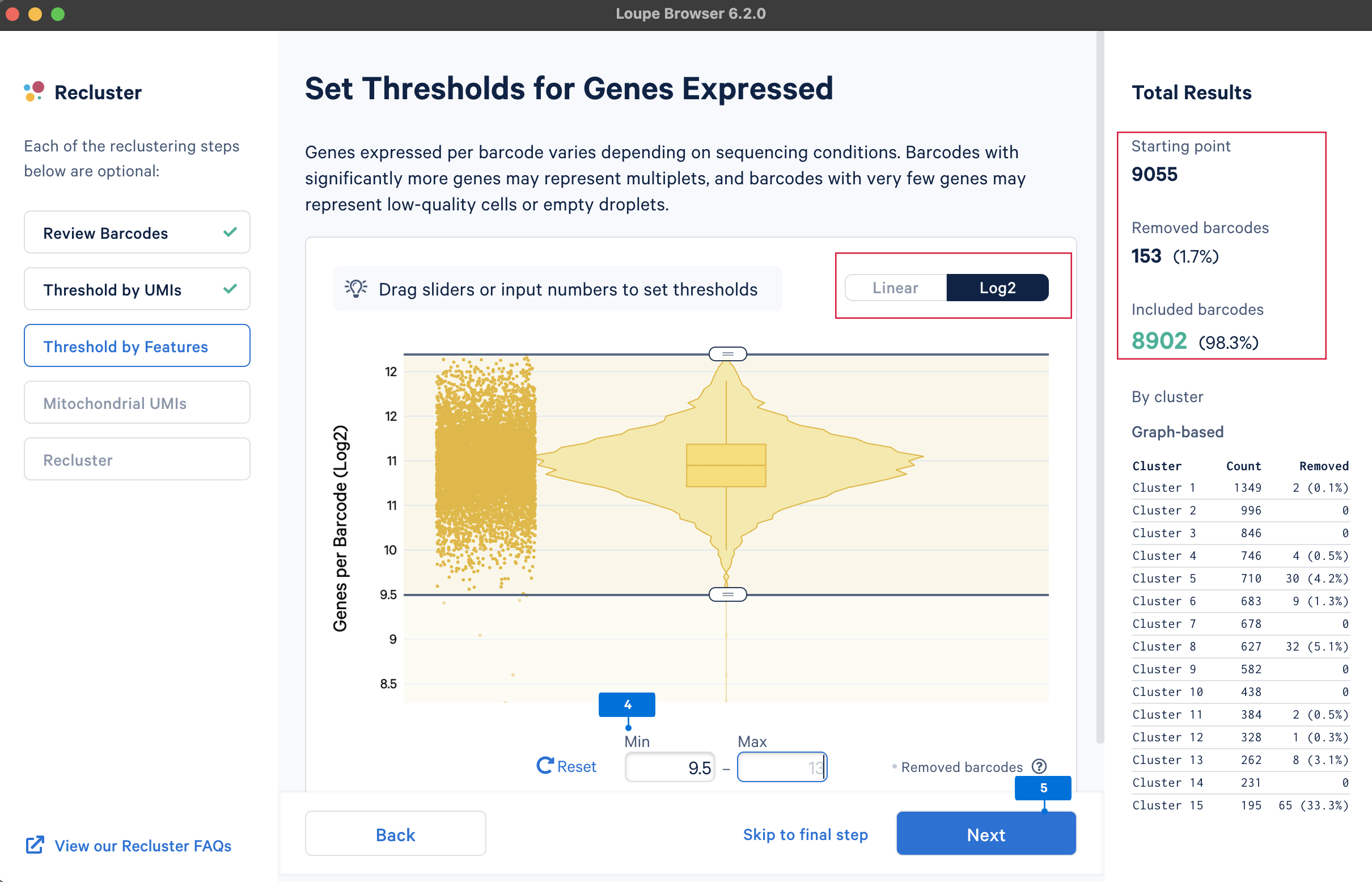
The main purpose of this step is to remove potential low-quality cells and multiplets. Similar to UMI counts, there are no universal QC rules on the number of detected genes. Here, select the barcodes with gene numbers between 29.5 and 213 (most of the cells are within this range).
A high level of mitochondrial gene expression could indicate dying cells (see this knowledge base article, Ilicic et al. 2016). QC filtering based on mitochondrial gene levels could remove these low-quality cells. To filter barcodes based on mitochondrial gene levels, the first step is to provide a list of mitochondrial genes. The gene lists for human and mouse are available in the pre-built references drop-down menu. Users can also upload custom mitochondrial gene set lists for different species or other gene sets of interest, such as the ribosomal genes.
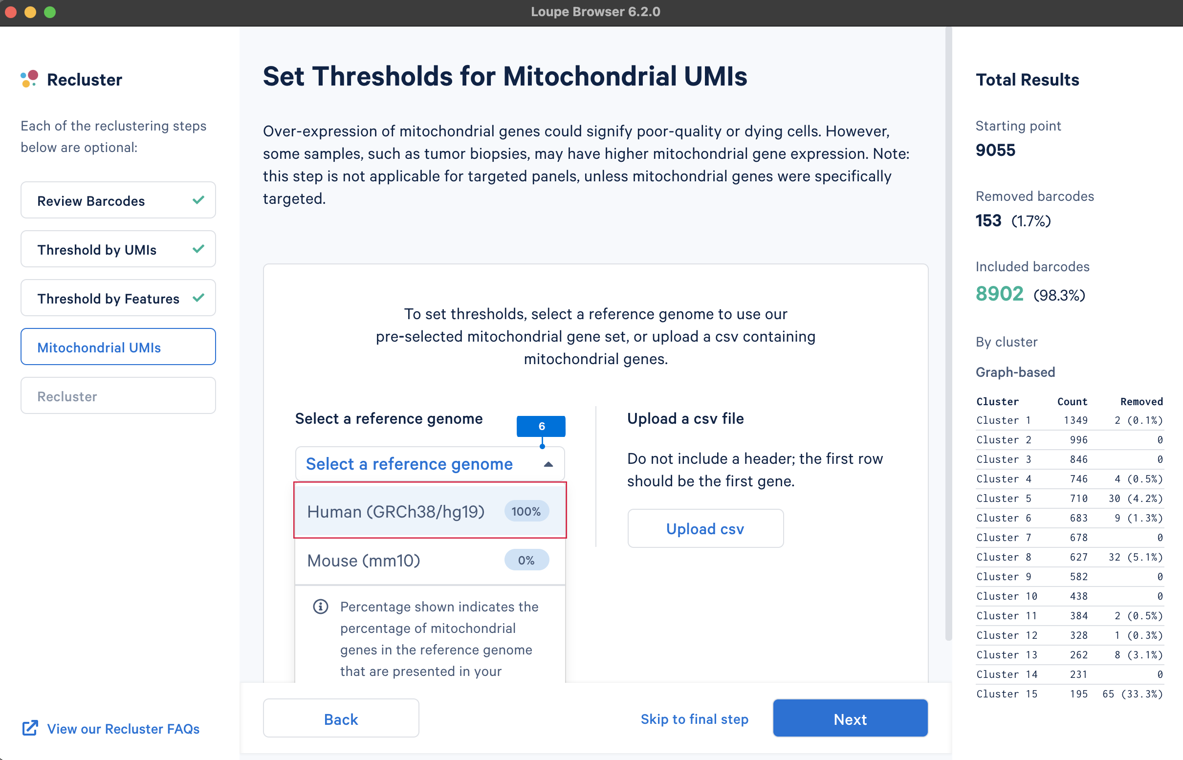
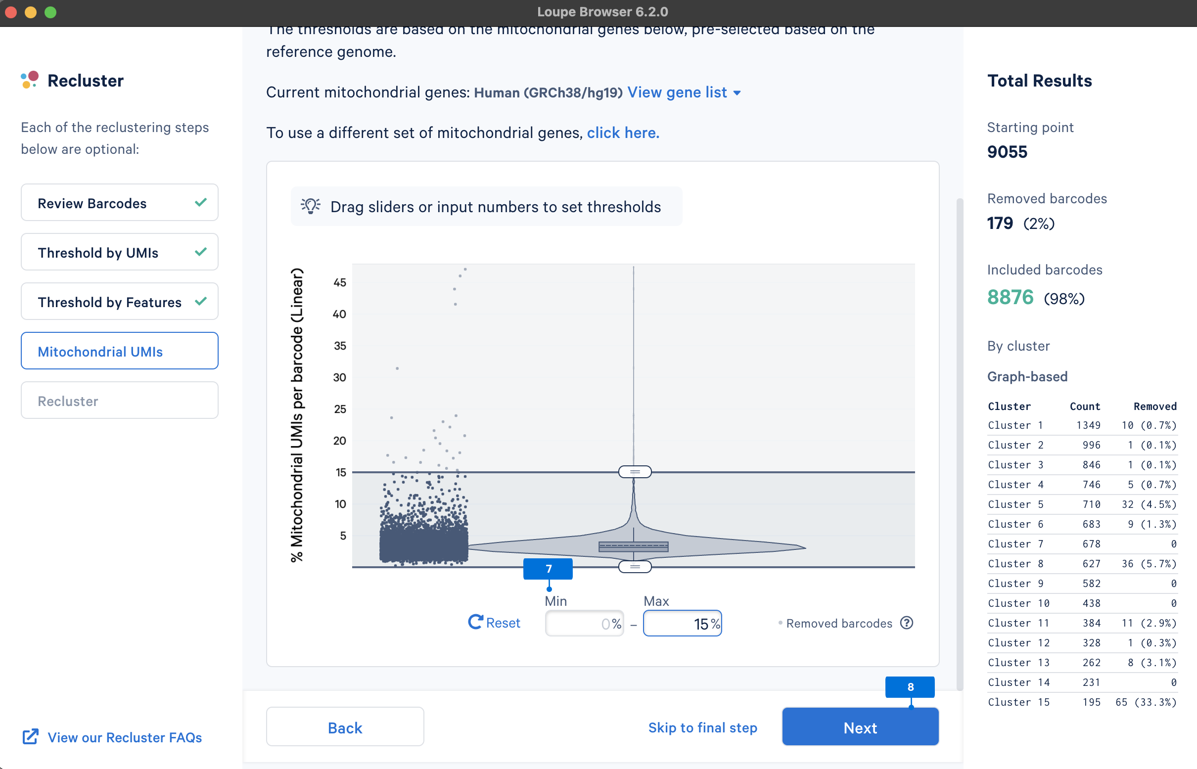
Similar to the QC on UMI counts and the number of detected genes, there are no universal thresholds for the percentage of mitochondrial genes. If a review of available scientific literature suggests the study sample is known to have high mitochondrial gene expression (e.g., tumor biopsies), you may want to select less stringent filtering values.
The last step is to perform reclustering and projection, selecting both t-SNE and UMAP embeddings. Loupe Browser also provides features to Adjust reanalyze parameters (for advanced users) for reclustering and projection. This tutorial uses default parameters.
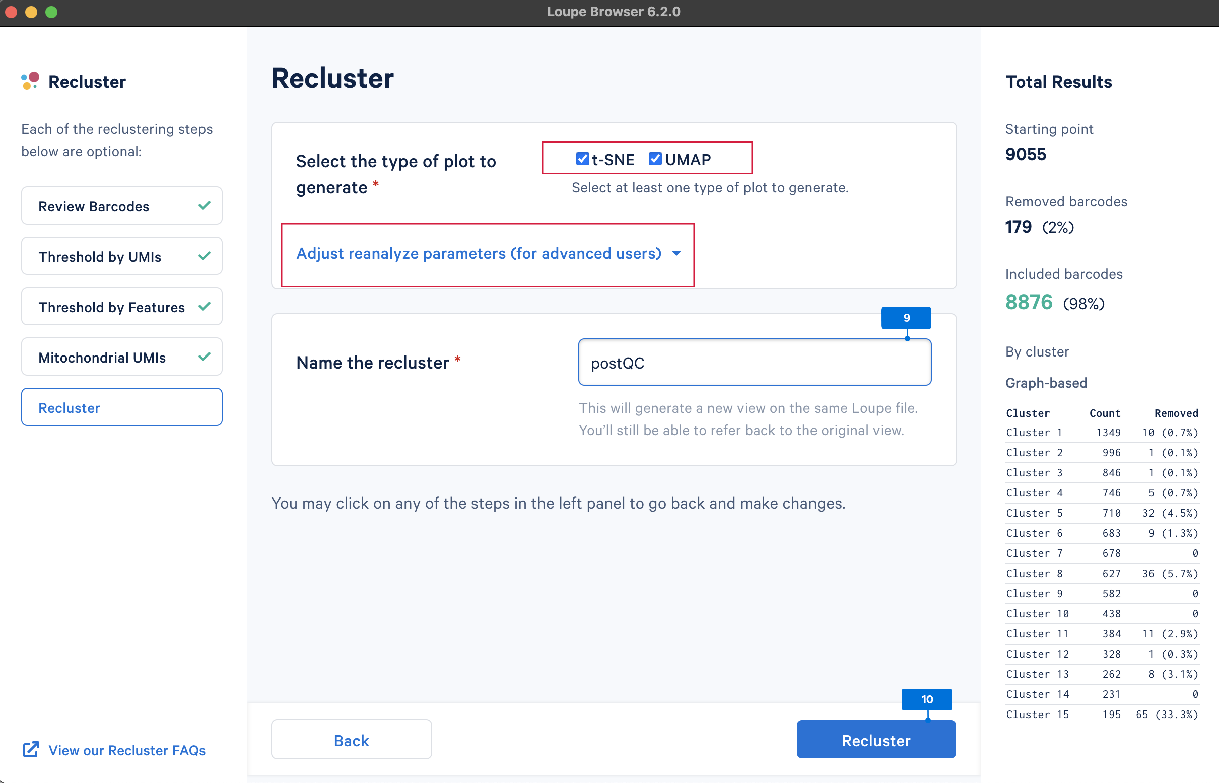
It takes several minutes to complete the reclustering. When complete, click Done to return to the Loupe Browser window.
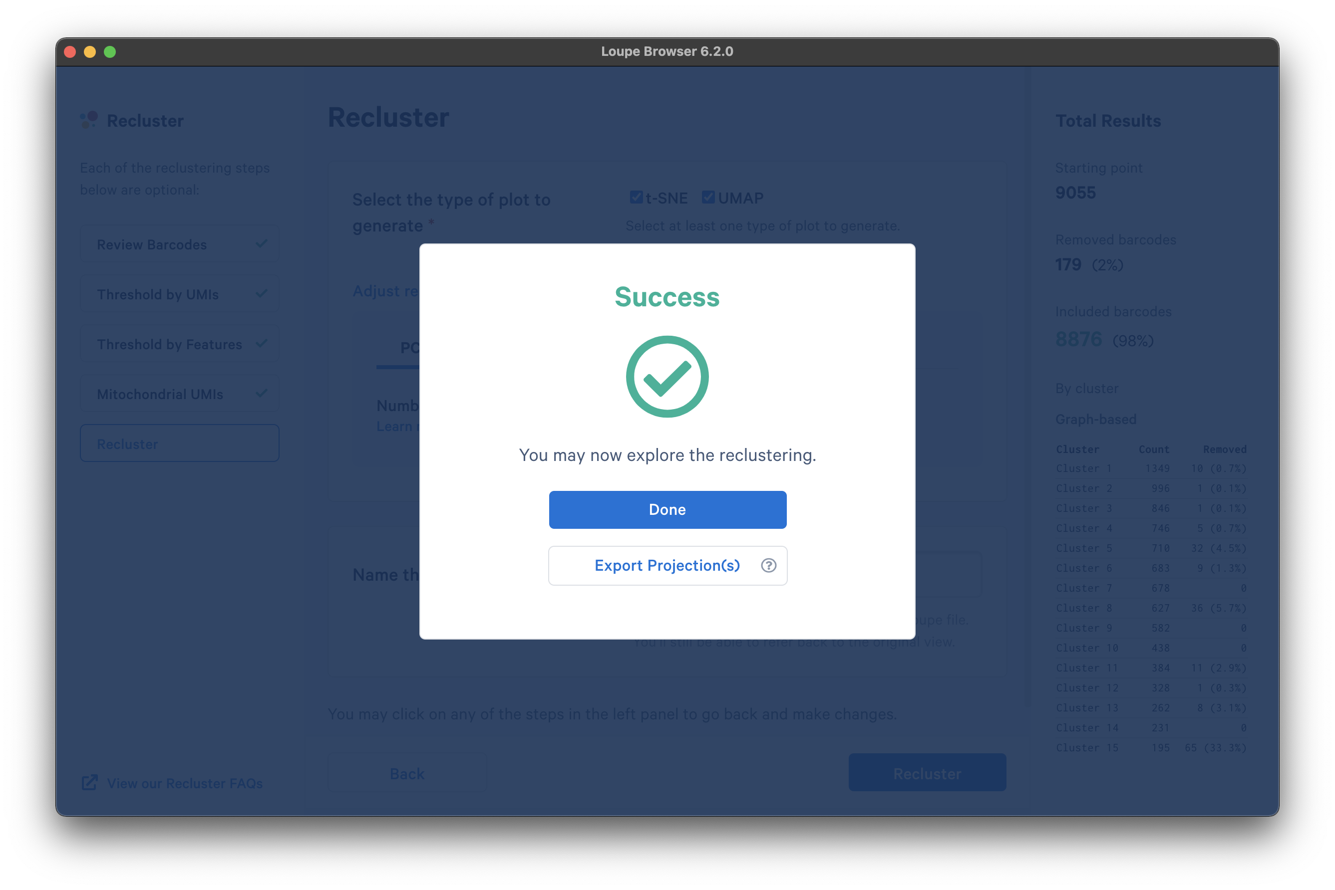
There are now new t-SNE and UMAP plots ("postQC" Category label) generated from the reclustering results for our post-QC cells.
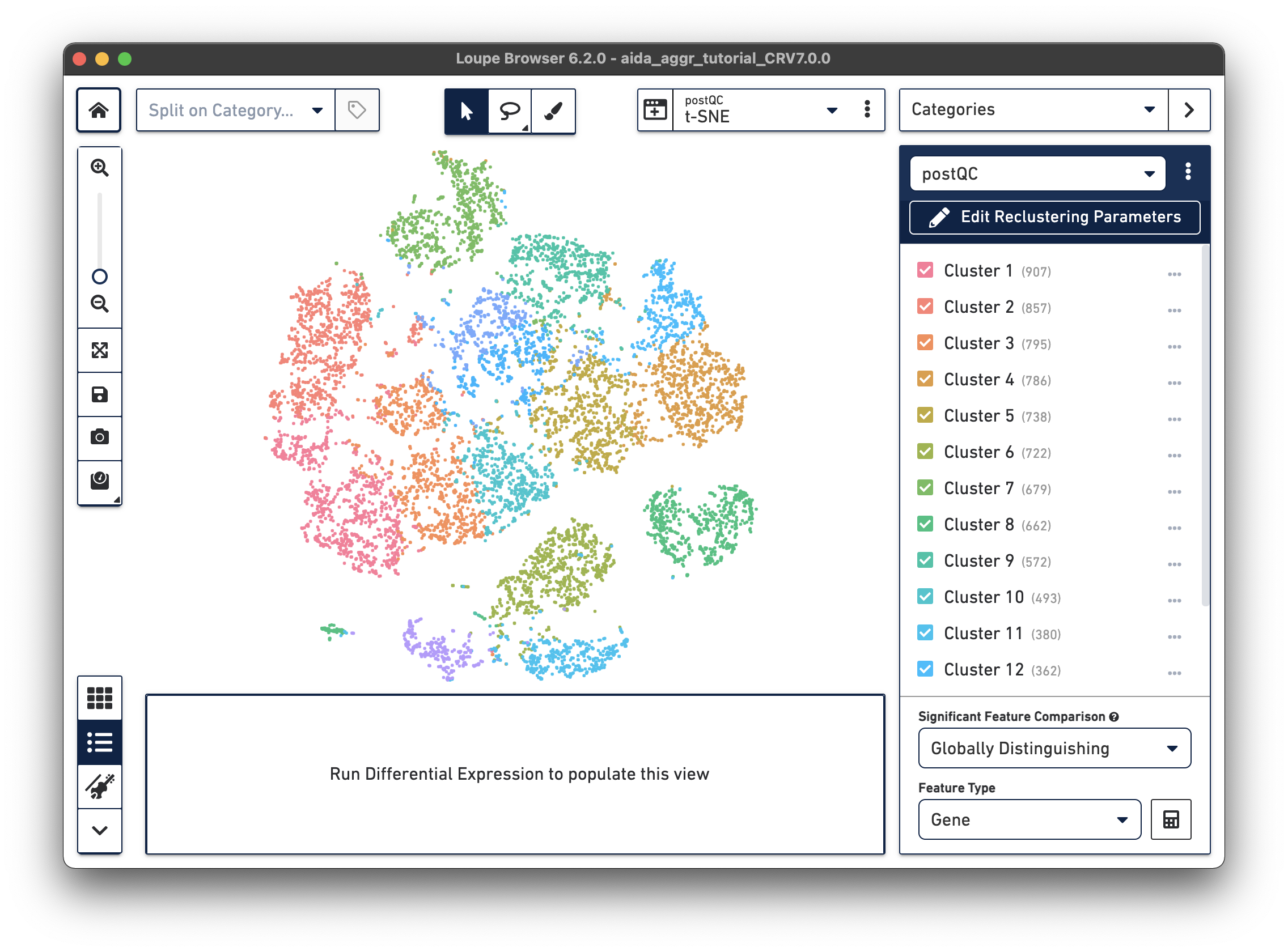 |
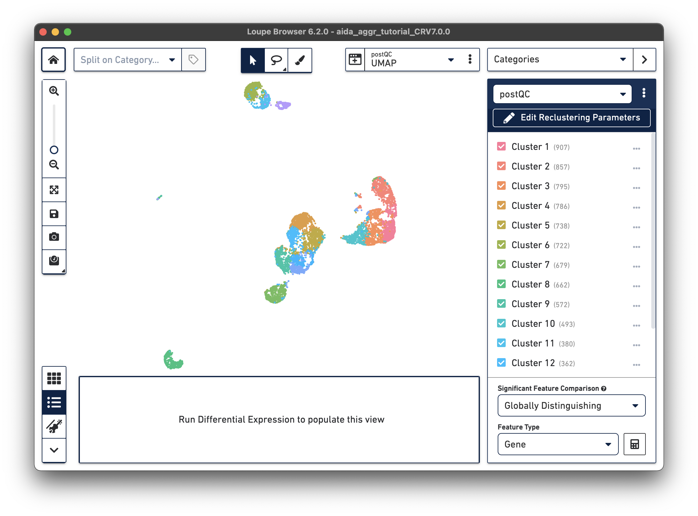 |
After obtaining clusters based on gene expression similarity, identify the corresponding cell type for each cluster. This cell annotation process can be challenging. For more information, see this cell type annotation tutorial in Loupe Browser and this Analysis Guide that describes several additional web resources for cell annotation.
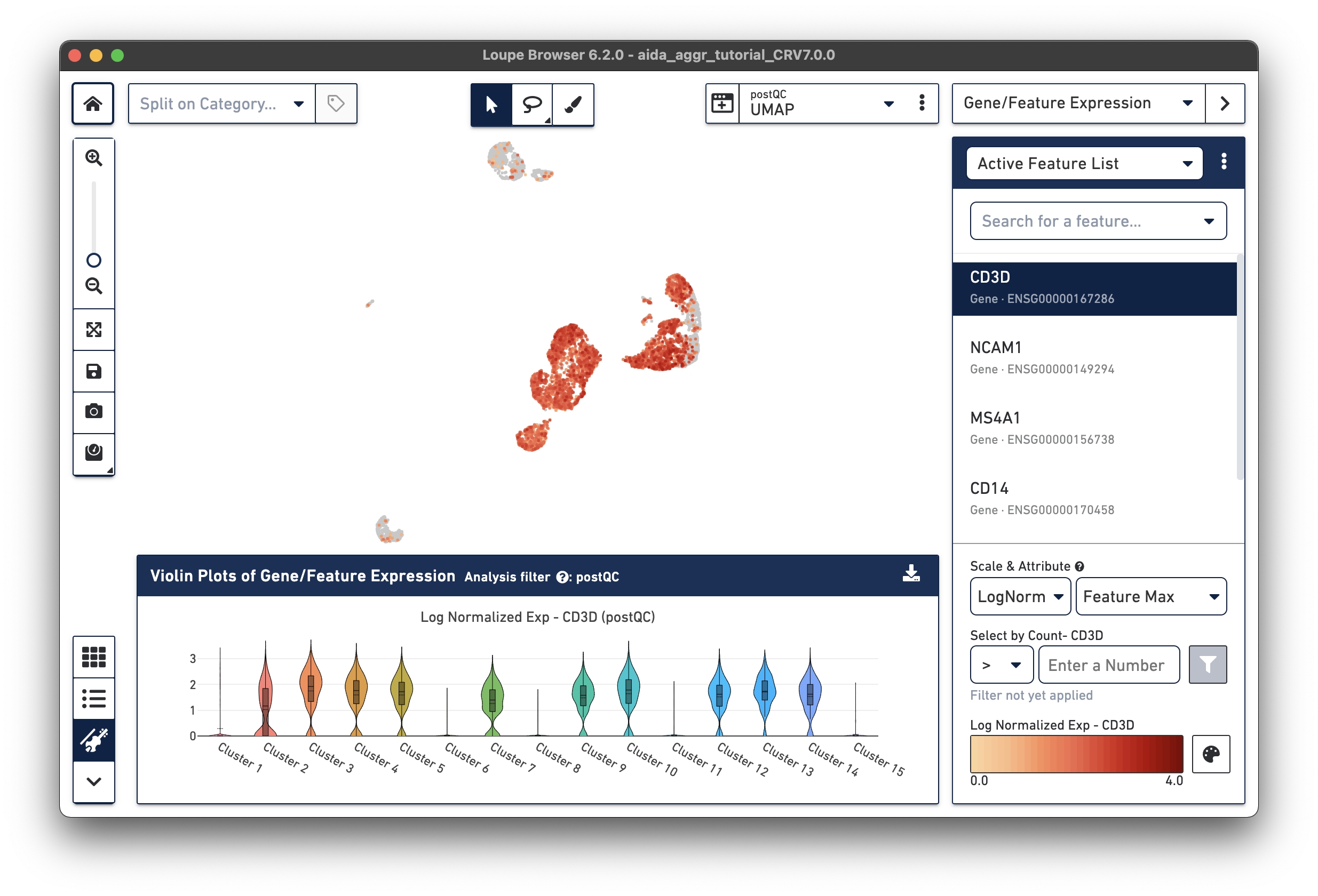
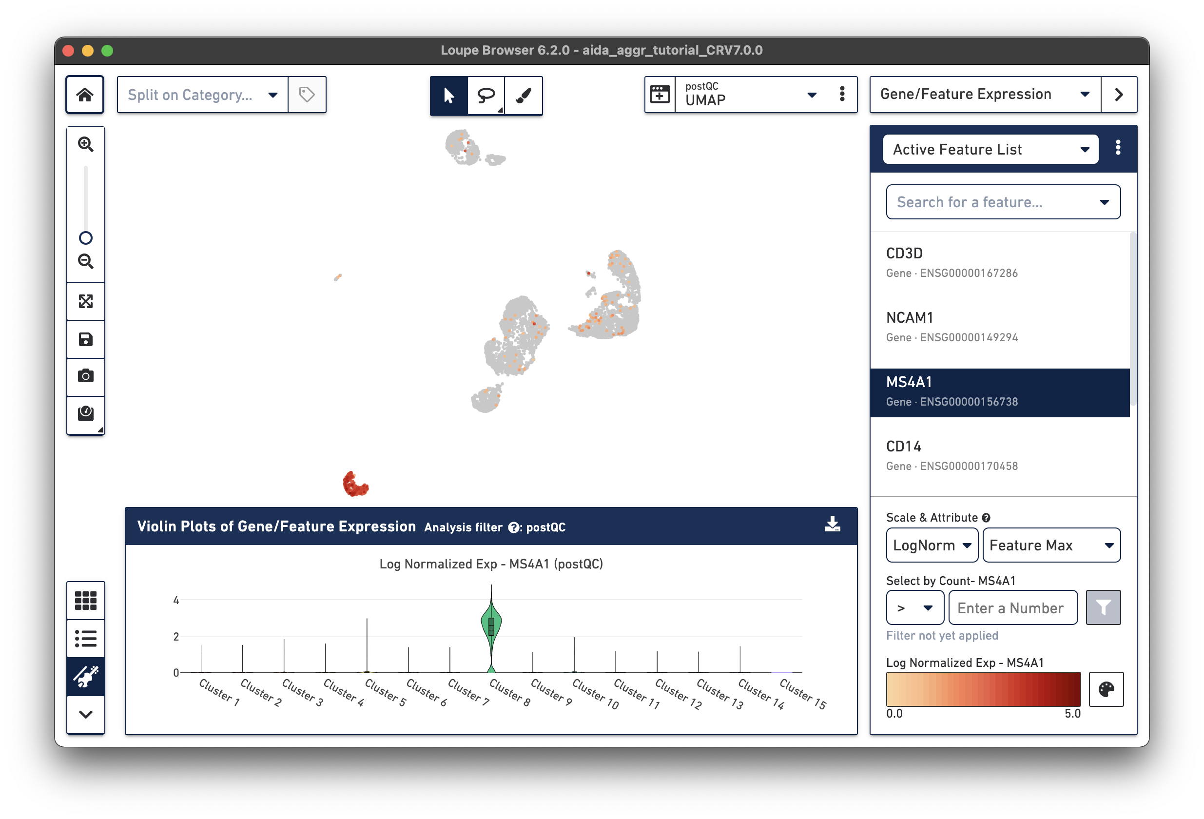
This tutorial uses marker-gene-based manual annotation to identify the major peripheral blood mononuclear cell (PBMC) cell types (the Split on Category view and Lasso Selection tool can also be used to annotate cell clusters). The Gene/Feature Expression top-right panel of Loupe Browser allows researchers to profile gene expression across cells. The Feature Plot function enables visualization of the expression levels for key PBMC marker genes across all cells in the dataset. Finally, the gene expression levels in different clusters can be visualized with Loupe Browser's violin plot function.
Based on the expression levels of key PBMC marker genes across clusters, these clusters can be annotated into major immune cell types: T cells, NK cells, B cells, and monocytes. In particular for monocytes, based on the relative expression levels between CD14 and FCGR3A (CD16), two monocyte subtypes, i.e. CD14 monocyte (classical) and CD16 monocyte (non-classical), can be further characterized. Click the tabs below for each cell type:
Here, observe that CD3D, a marker for T cells, is expressed in Clusters 2-5, 7, 9, 10, and 12-14 in the violin plots. We will use these marker genes to annotate clusters by cell type.
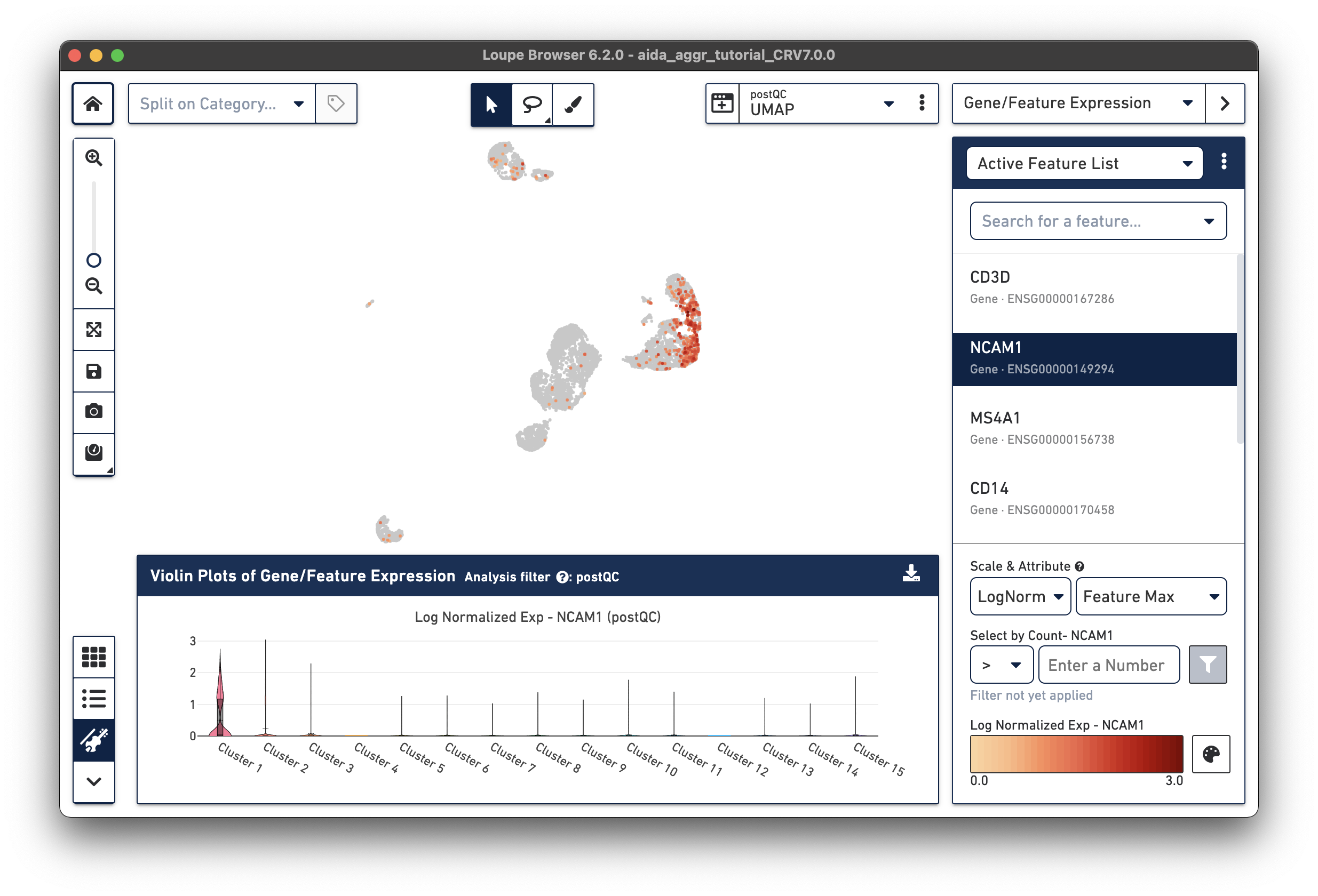
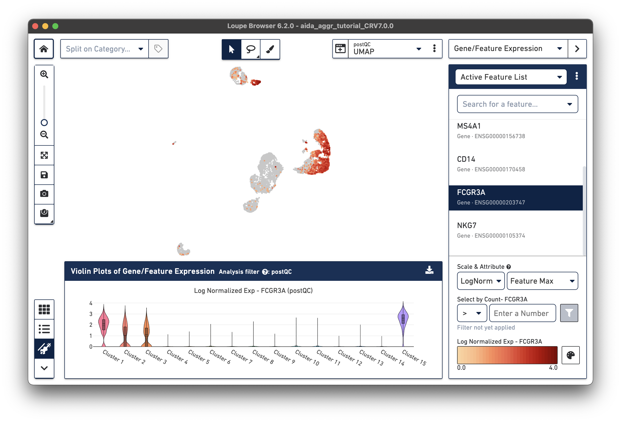
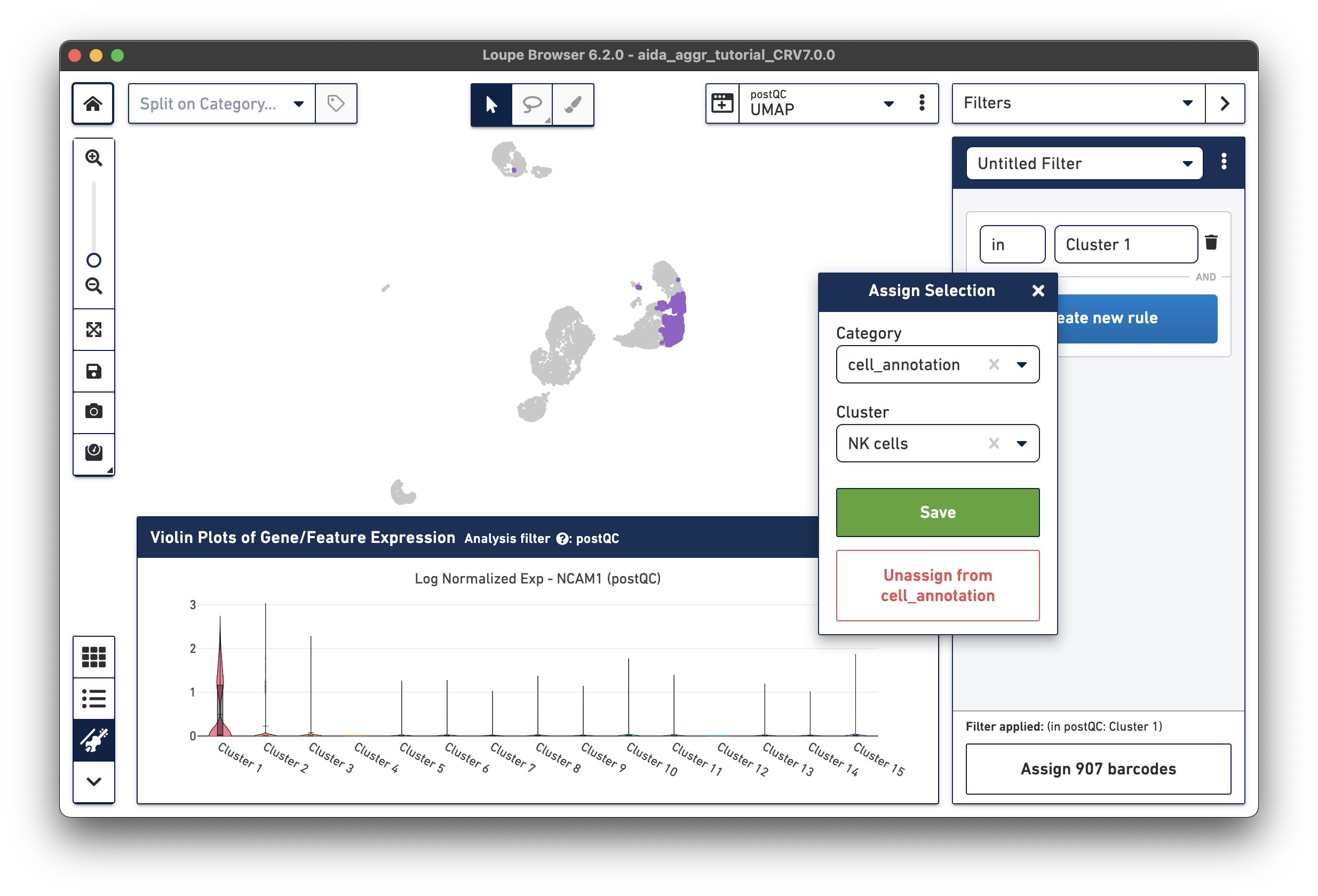
The marker gene for NK cells, NCAM1, is expressed in Cluster 1. While less NK cell-specific, NKG7 and FCGR3A can also be used to support NK cell annotation as they characterize NK cell cytotoxic functions (the violin plot gene expression patterns will shift as you select each gene from the Active Feature List).
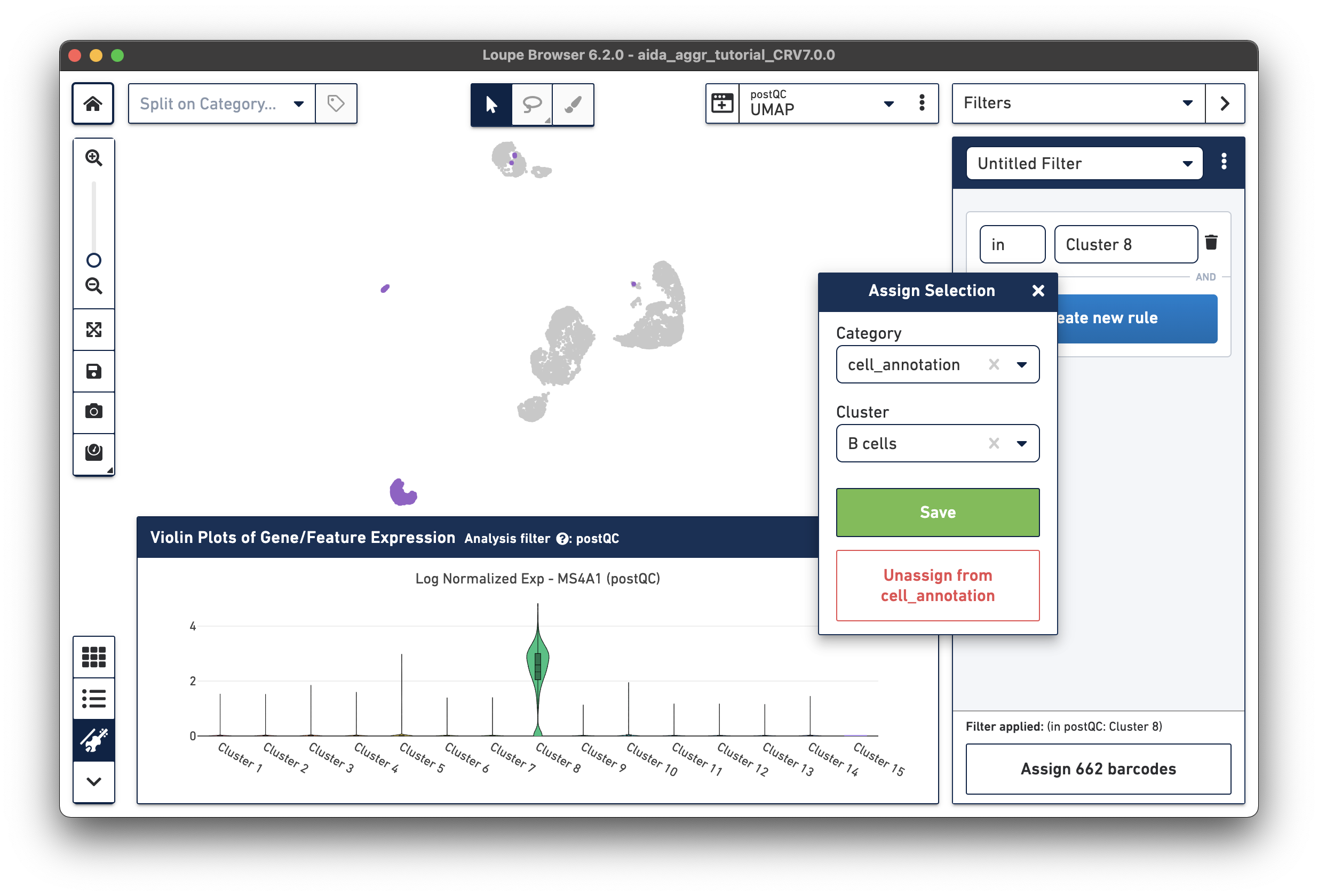
The marker gene for B cells (MS4A1) is expressed in Cluster 8.
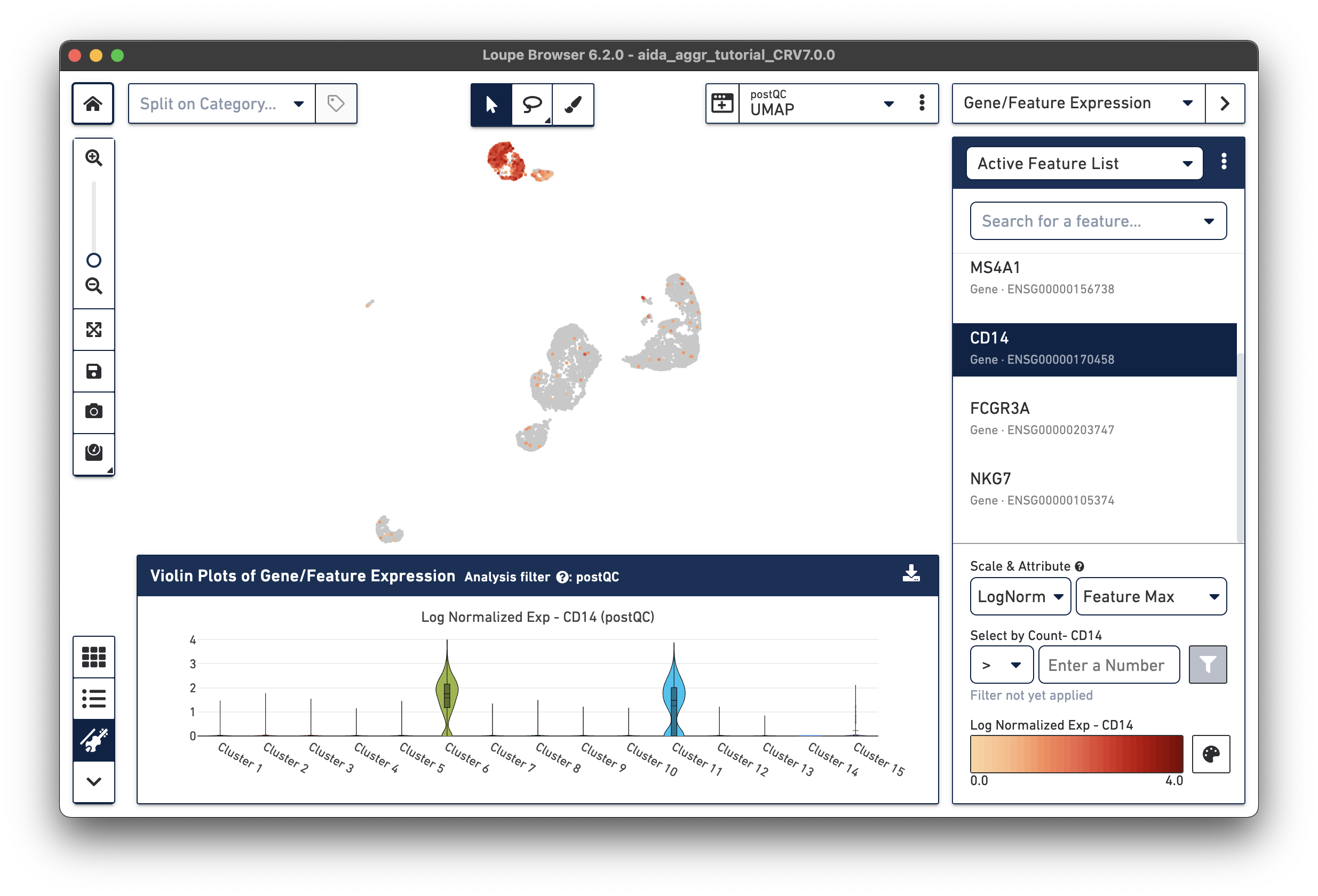
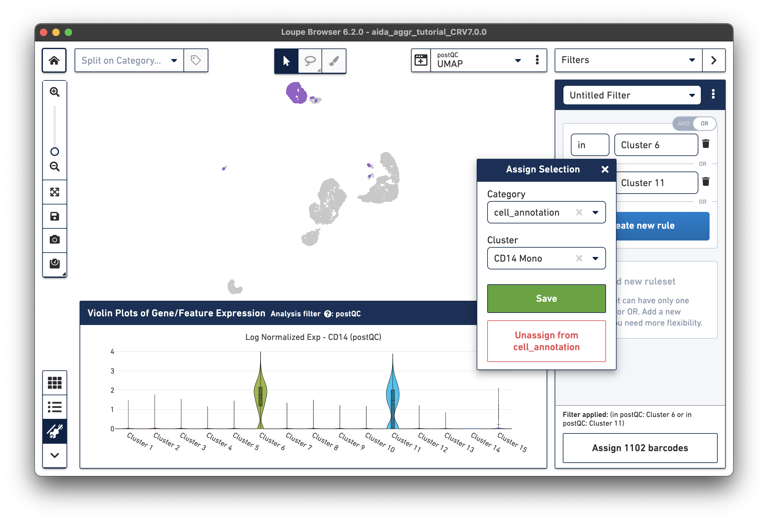
The marker genes for CD14 monocytes (CD14high, FCGR3Alow) are expressed in Clusters 6 and 11.
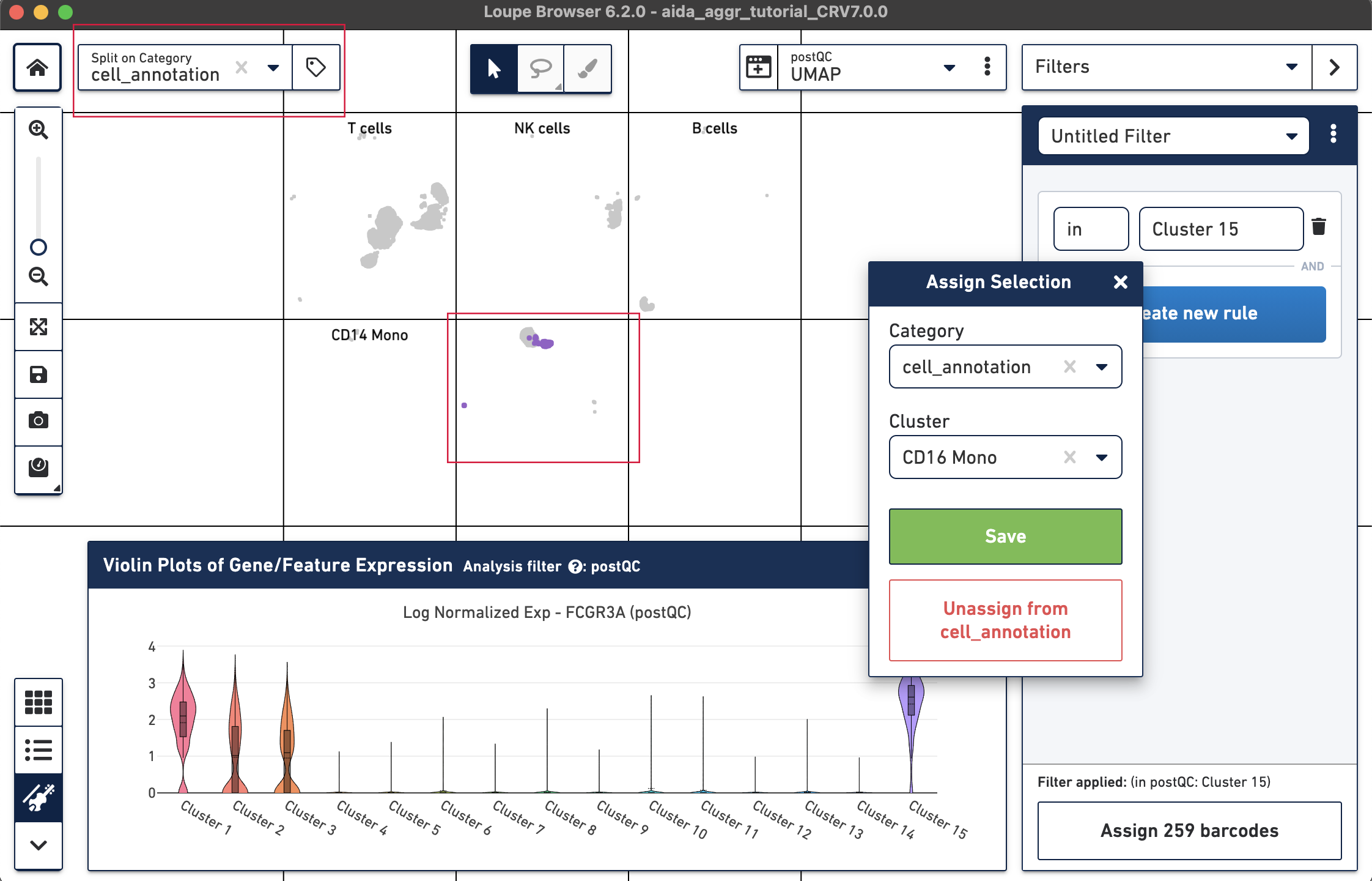
The marker genes for CD16 monocytes (CD14low, FCGR3Ahigh) are expressed in the remaining cluster, Cluster 15.
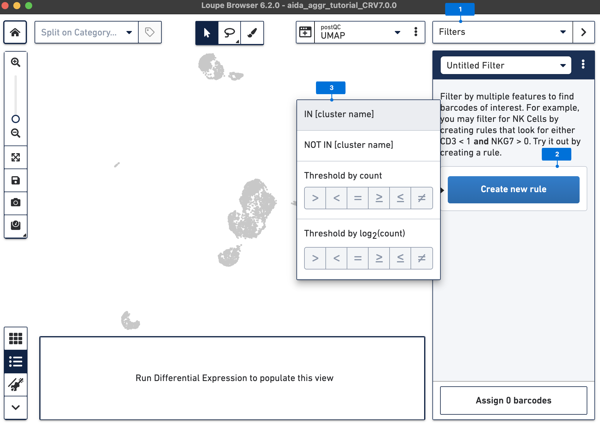
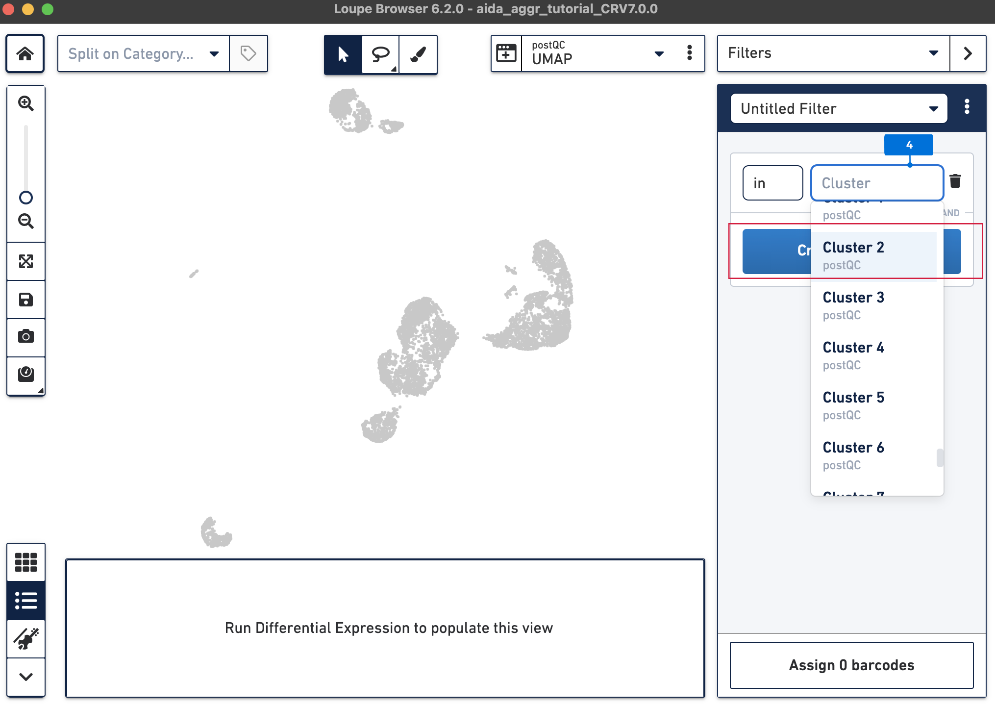
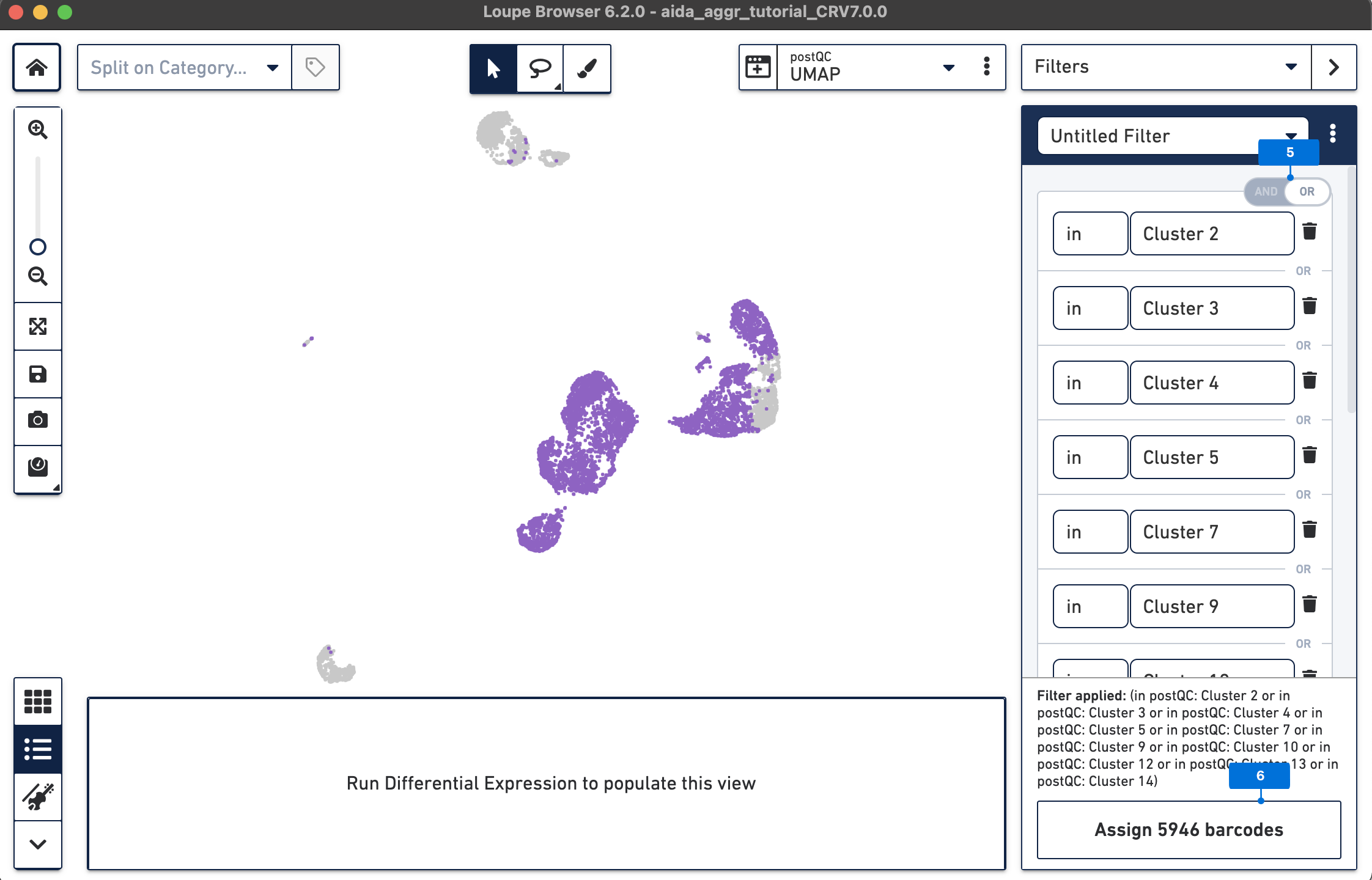
The Filters function on the top-right panel of Loupe Browser can now be utilized to annotate each cluster. Begin by annotating Clusters 2-5, 7, 9, 10, and 12-14 as T cells. Note that these different clusters in T cells could represent different T cell subtypes (not discussed in this tutorial, for cell subtype annotation, see this tutorial).
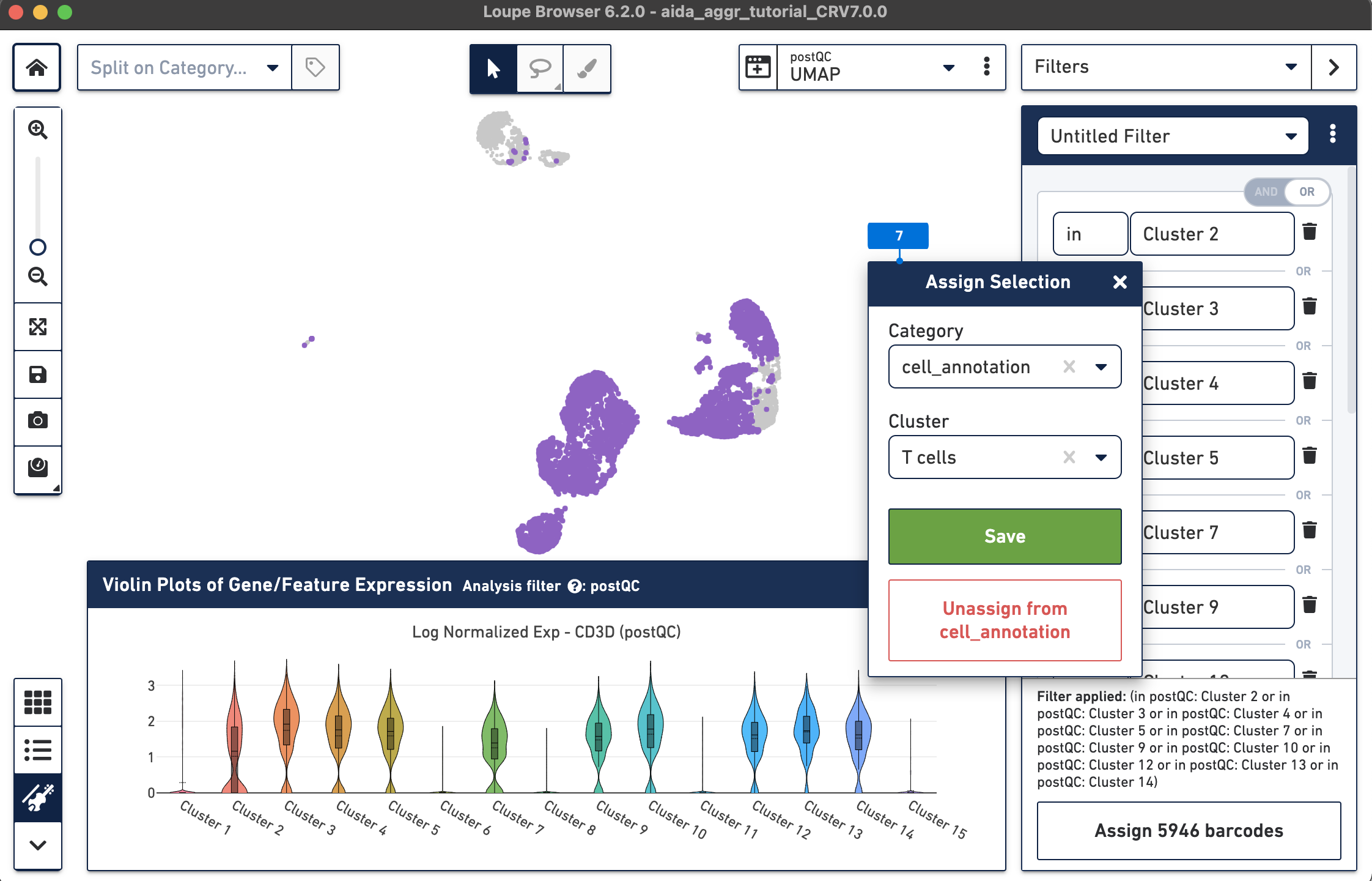
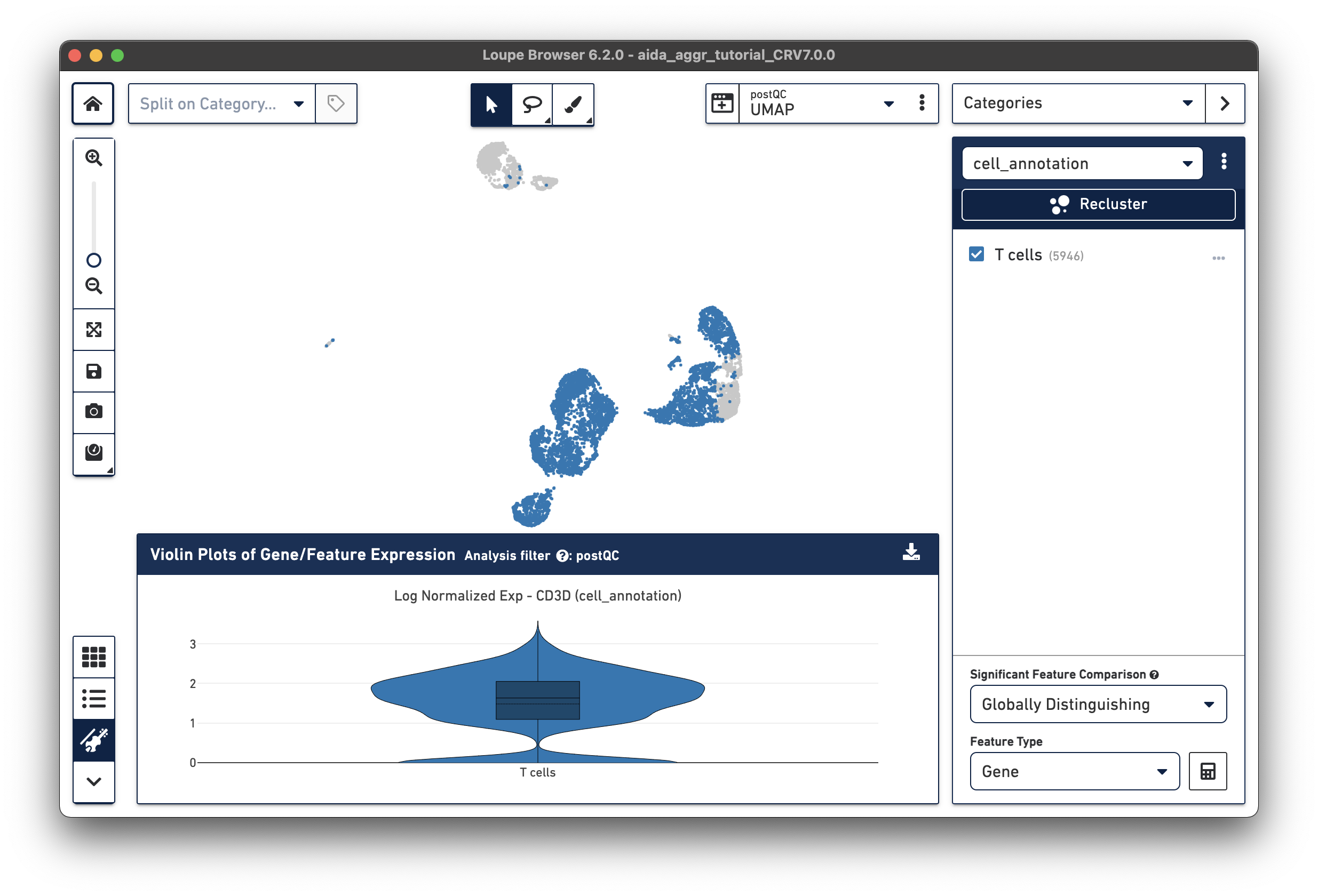
The T cell annotation is now added to the Categories panel under "cell_annotation".
Assign the remaining clusters using the Filters option (delete previous cluster rules using the trash bin icon) - click the tabs below for each cell type:
Based on the expression levels of CD14, the unannotated clusters 6 and 11 are identified as CD14 monocytes:
Now that we have annotated several clusters, use the Split on Category option to display the UMAP projection split by cell annotation. Based on the expression levels of CD16, the unannotated cluster 15 is CD16 monocytes:
Now all the major PBMC cell types are annotated:
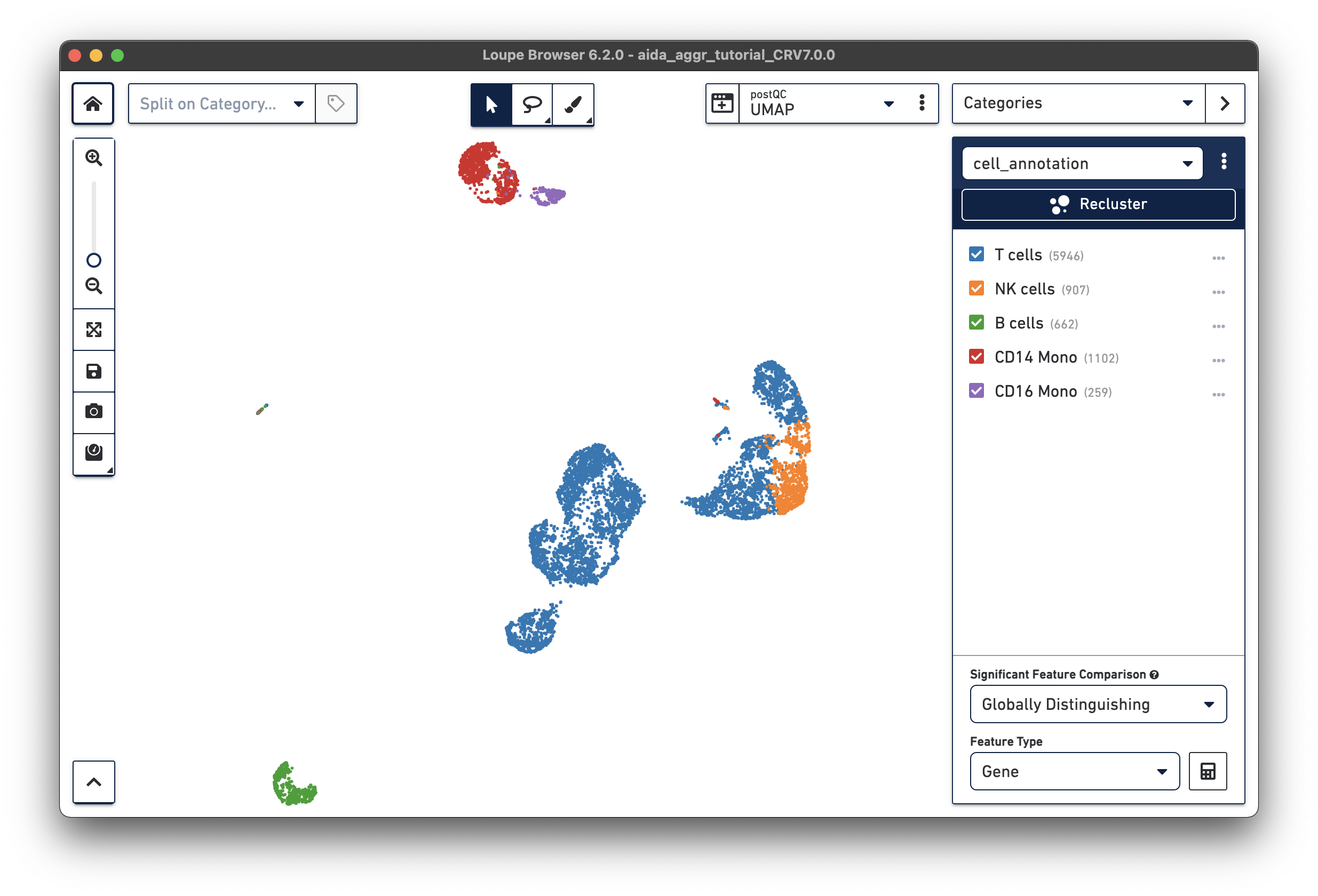
Based on the marker gene expression profiles, clusters are annotated in major PBMC cell types. The cell annotation results can be exported as a CSV file with the annotation for each barcode (export with unlabeled or only labeled barcodes).
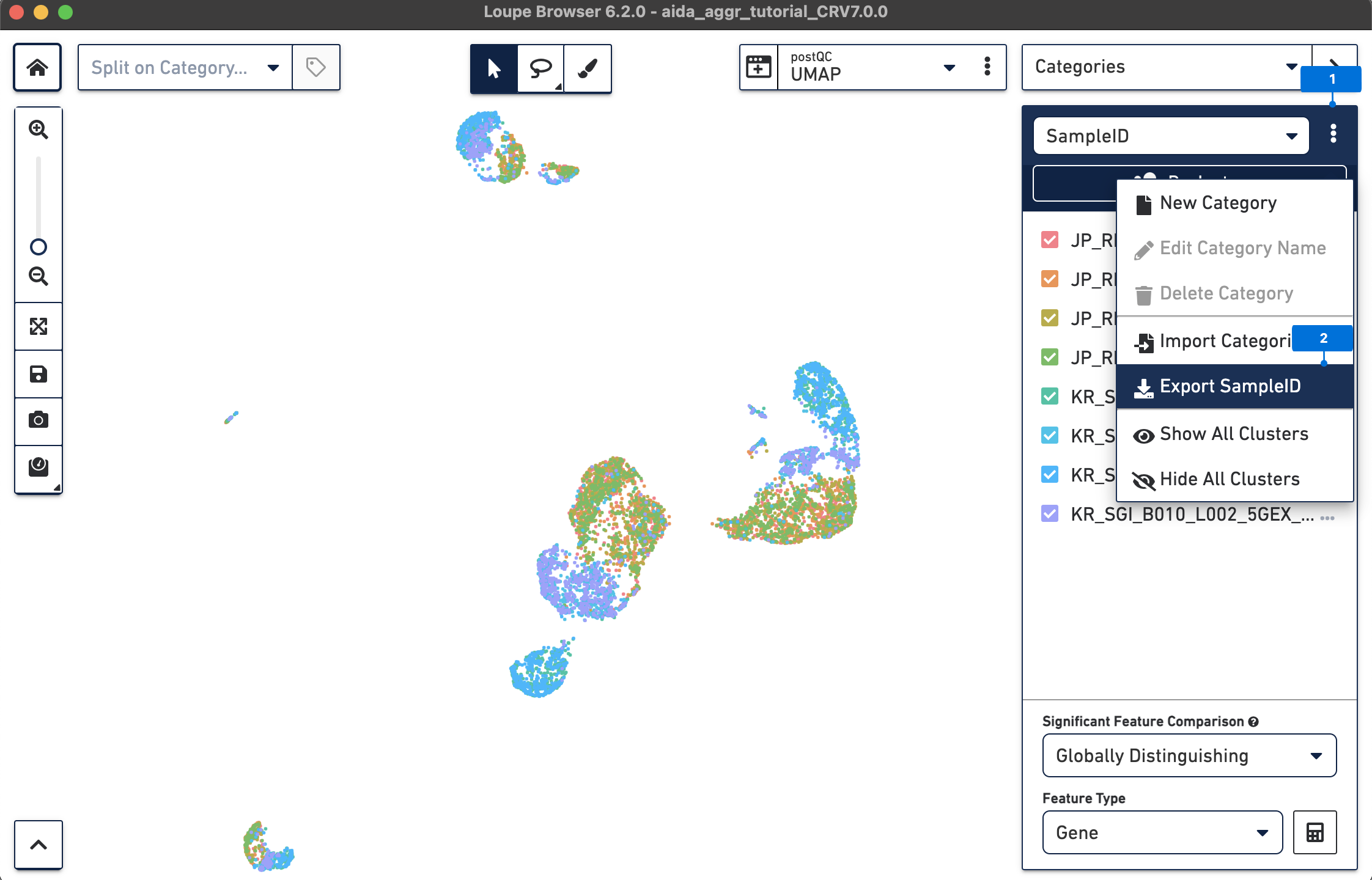
Loupe Browser supports the import of metadata as new categories, such as donor and country in this case study. Accordingly, differentially expressed gene analysis can be performed based on the new metadata. Below, two methods are illustrated to import new metadata either manually from the exported SampleID category or by using Filters to annotate samples.
Here, since the information of donor and country is based on sampleID:
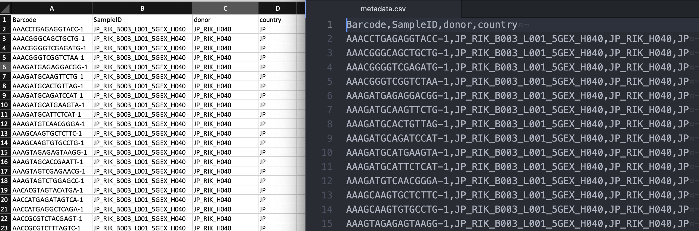
Next, based on sampleID, add the information of donor and country for each barcode in a text editor such as Excel:
Save the table as a comma-separated value (CSV) file (metadata.csv) (left: Excel, right: text editor view of the CSV format):
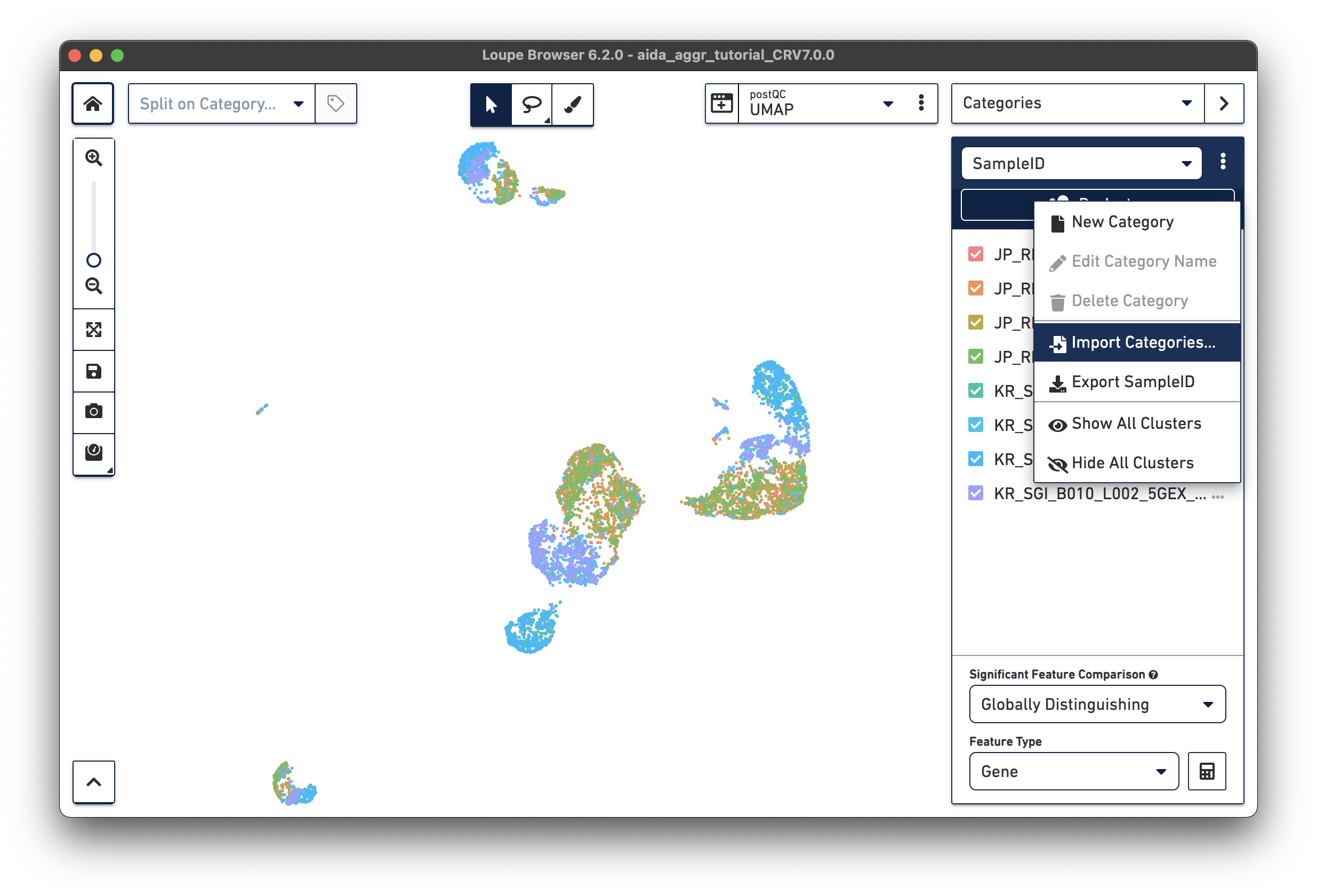
Import the metadata file into Loupe Browser as a new category (this file is also provided for download in Data overview):
The split view by sampleID enables another way to select samples for category assignment. In the Filters panel, cells in JP_RIK_B001_L001_5GEX_H040 and JP_RIK_B001_L002_5GEX_H040 are assigned to cluster JP_RIK_H040 in the donor category. A similar strategy is applied to the other three donors, as illustrated in this video:
Similarly, the Filters function is utilized to group cells into different countries, as illustrated in this video:
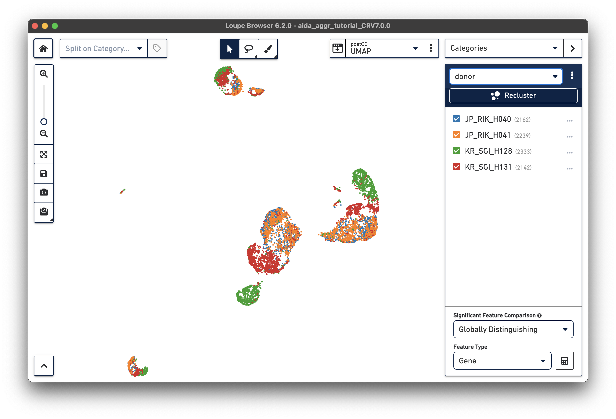
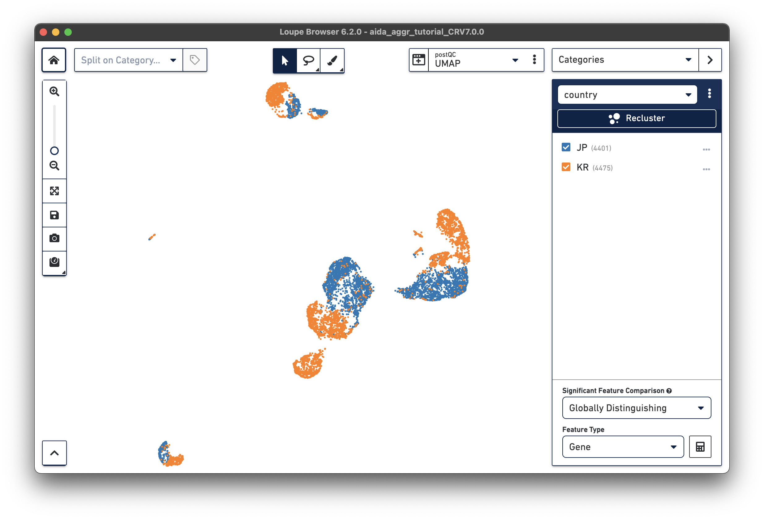
After either manually adding the donor/country categories or using the Filters function, two new categories are generated:
 |
 |
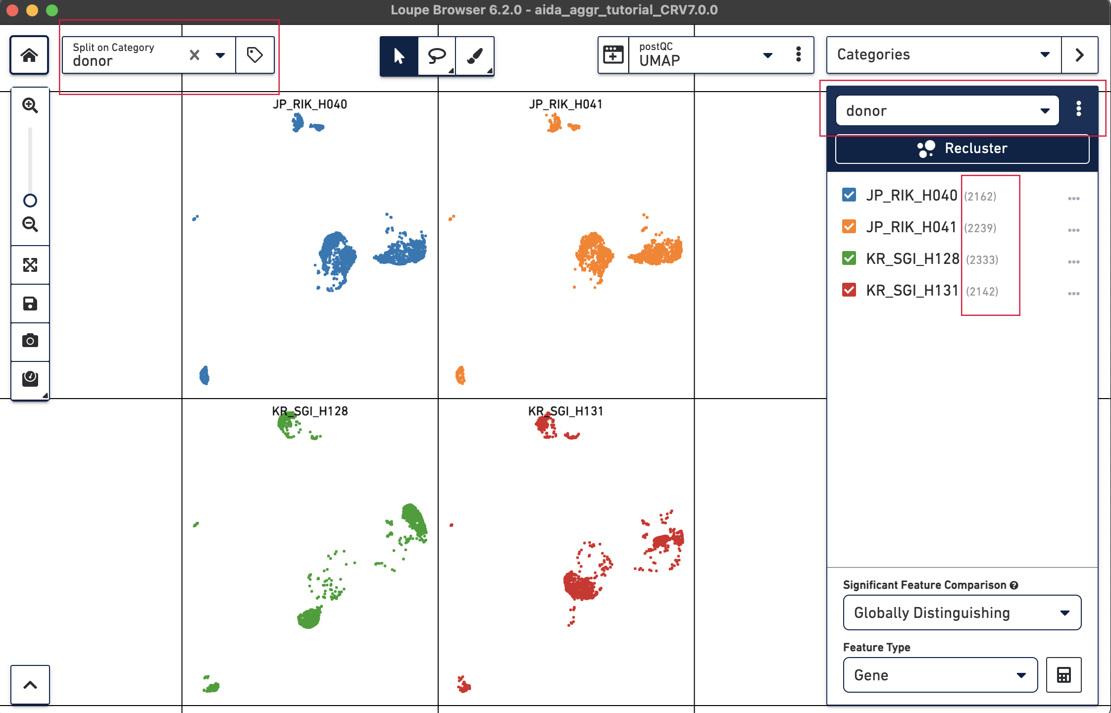
We will now compare the cell abundance of T cells across the four donors. The split view by donors shows their cell profiles in the UMAP plot (“donor” should be selected in “Categories”). From the donor category in the right panel, we can obtain the total cell number for each donor (e.g., 2,162 cells for donor JP_RIK_H040).
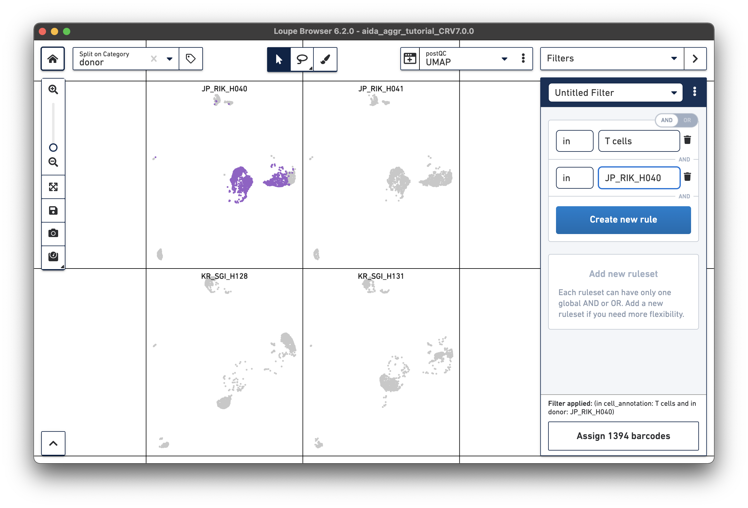
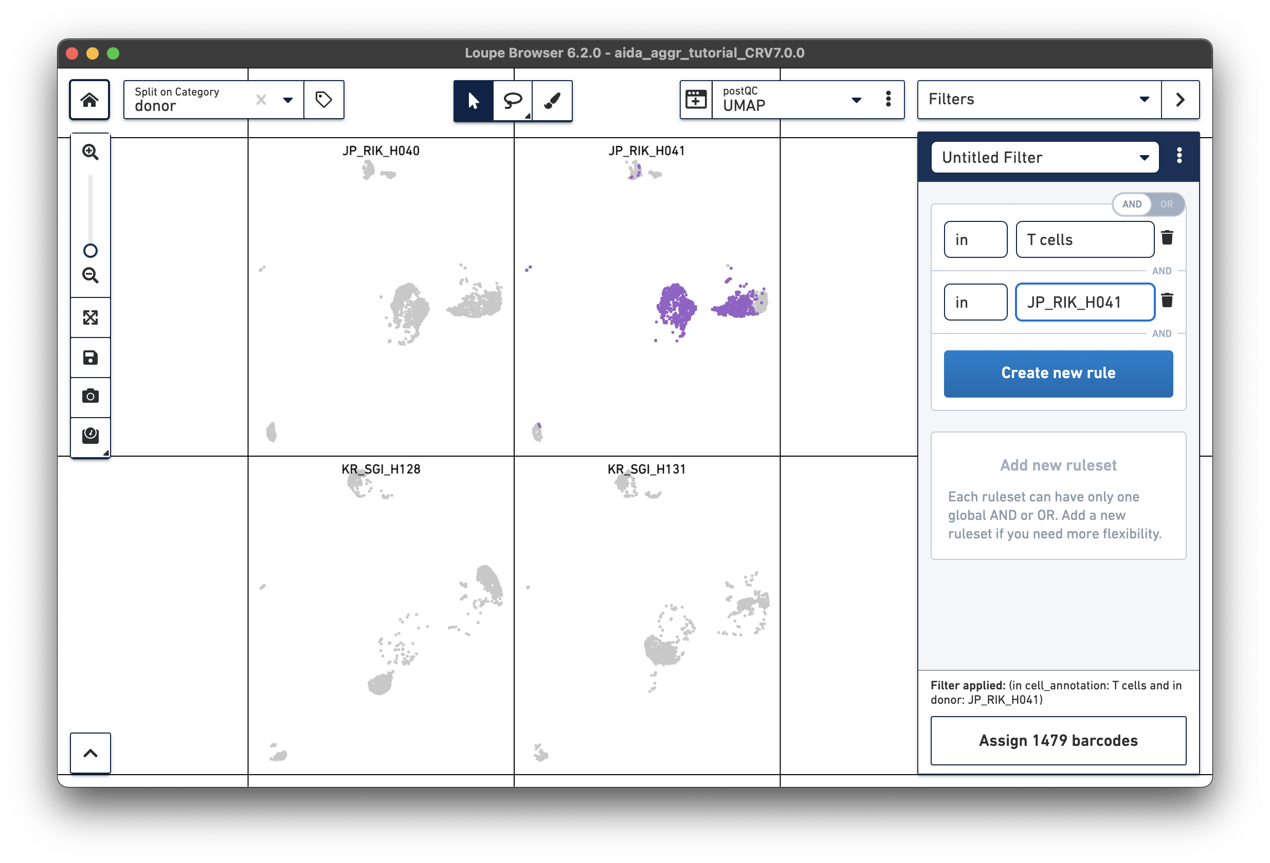
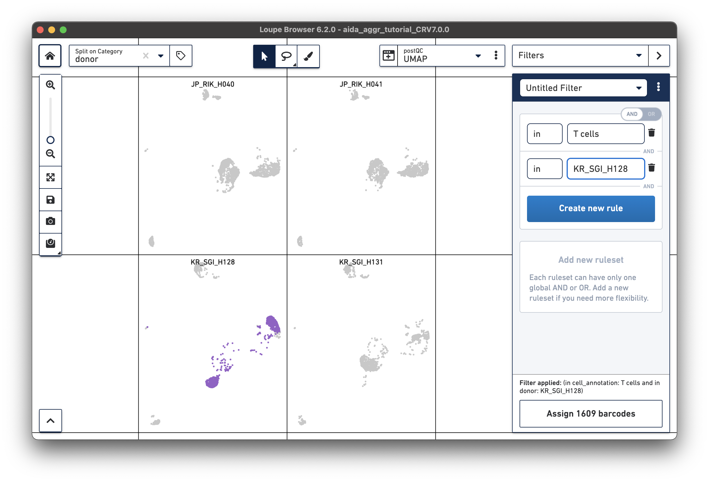
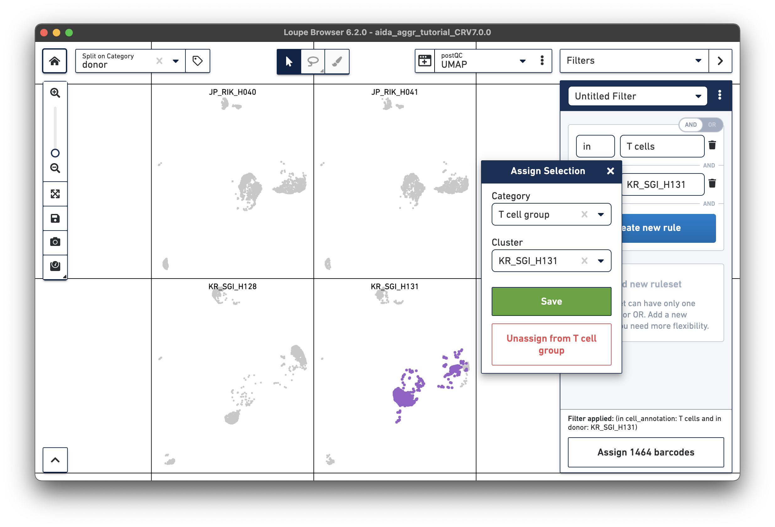
For the next step, the total T cell number will be counted for each donor in order to calculate the relative T cell ratio. The Filters function can be used to get the T cell number for each donor. Create a filter rule to select T cells for each donor as illustrated below (in this case, the AND/OR toggle should be set to AND). After setting the rules, T cell number for each donor will be shown at the bottom (e.g., 1,394 barcodes assigned to T cells for donor JP_RIK_H040).
  |
  |
Now, T cell abundance for the four donors can be calculated as below (the numerator comes from the filter for T cells by donor, the denominator from total cells per donor):
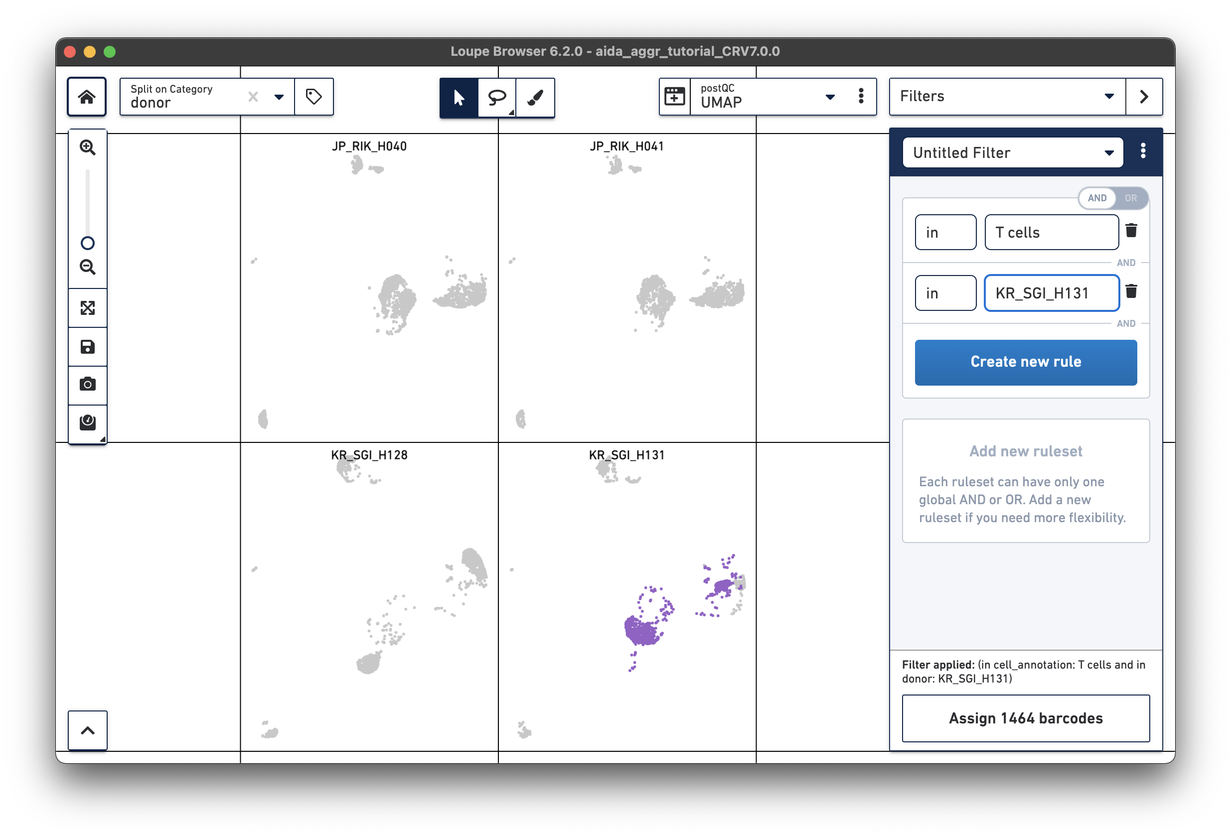
JP_RIK_H040 – 1394/2162 = 0.64
JP_RIK_H041 – 1479/2239 = 0.66
KR_SGI_H128 – 1609/2333 = 0.69
KR_SGI_H131 – 1464/2142 = 0.68
Loupe Browser provides the functionality to call differentially expressed genes (DEG) in globally and locally distinguishing modes. In the global mode, the DEG of each cluster vs. all the other clusters will be identified. In the local mode, the DEG will be called in a similar way to the global mode but only for the selected clusters. Here, DEG calling in T cells between the two South Korean donors, KR_SGI_H128 and KR_SGI_H131, will be performed to demonstrate this function in Loupe Browser.
Create a second filter rule for donor KR_SGI_H131:
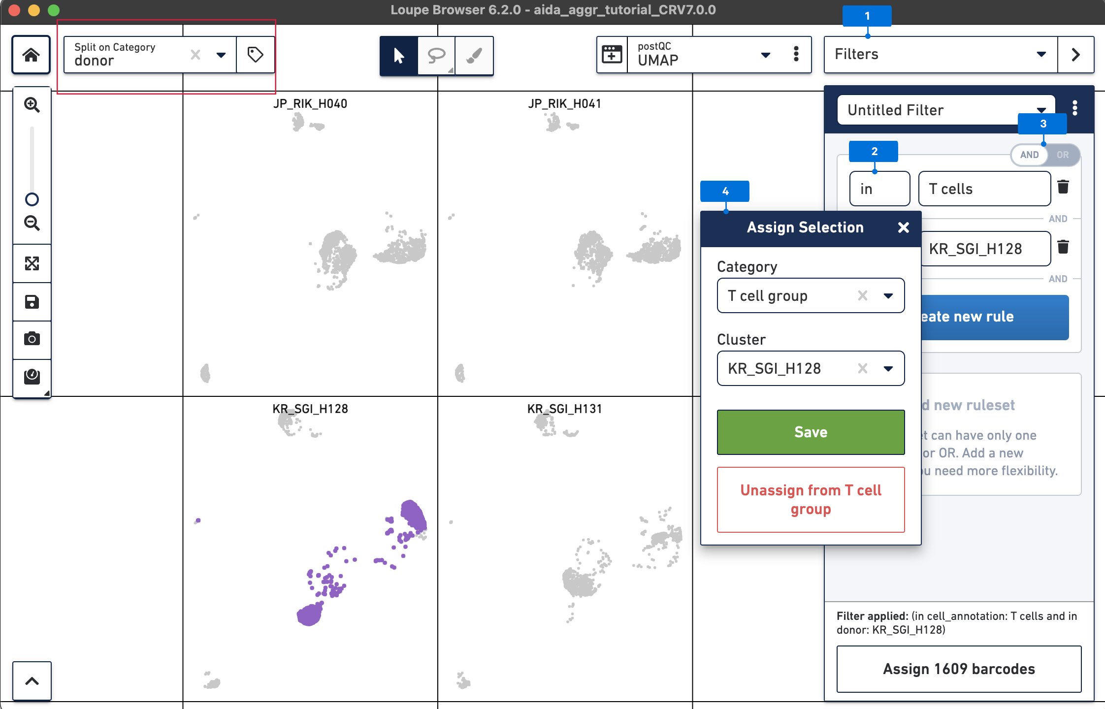
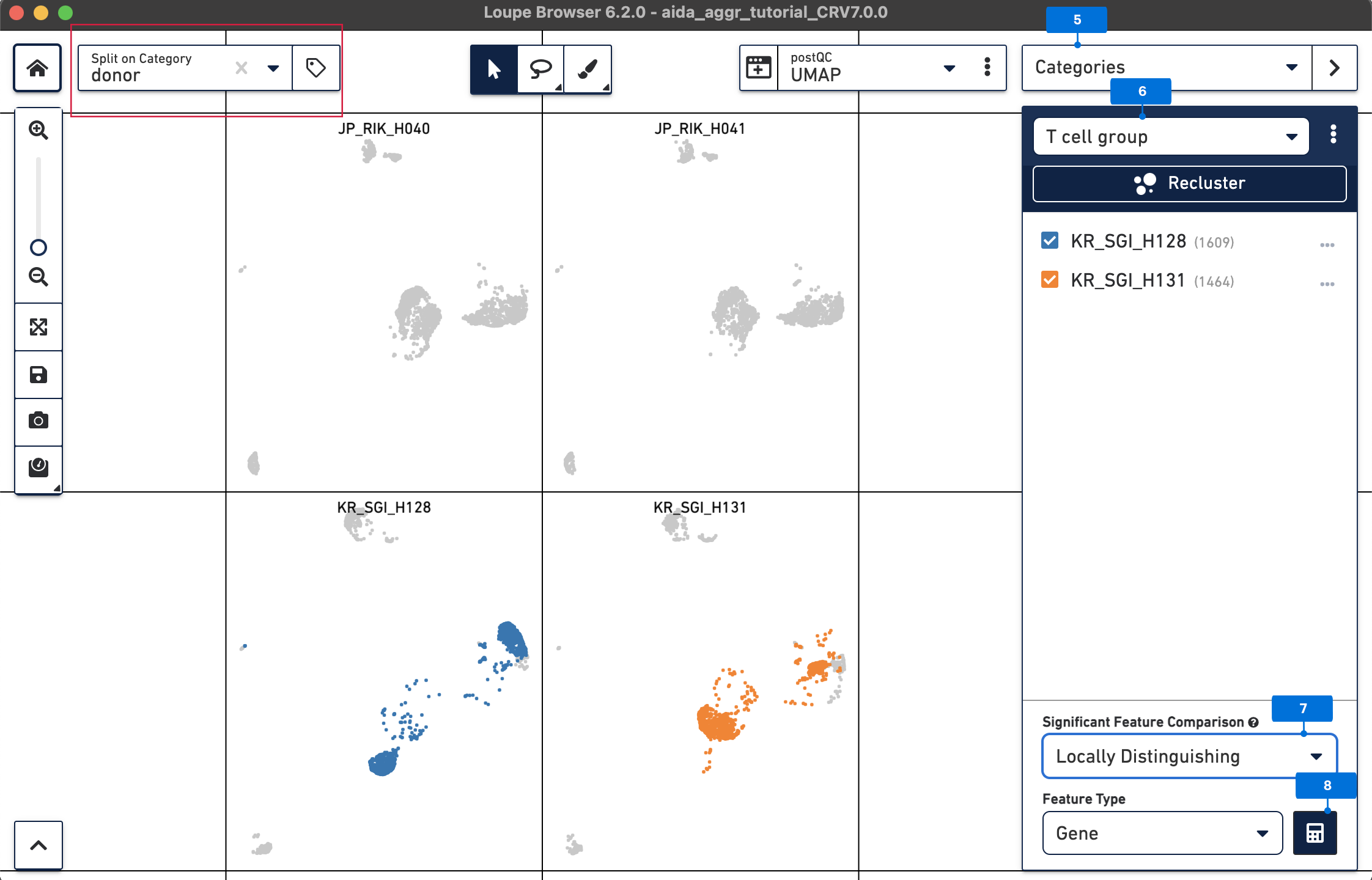
Now call differentially expressed genes: 5) Switch to Categories 6) Now T cells have been assigned to “KR_SGI_H128” and “KR_SGI_H131” clusters of new Category “T cell groups”. 7) Select Locally Distinguishing 8) DEGs in T cells between these two clusters can be measured by clicking the calculator button.
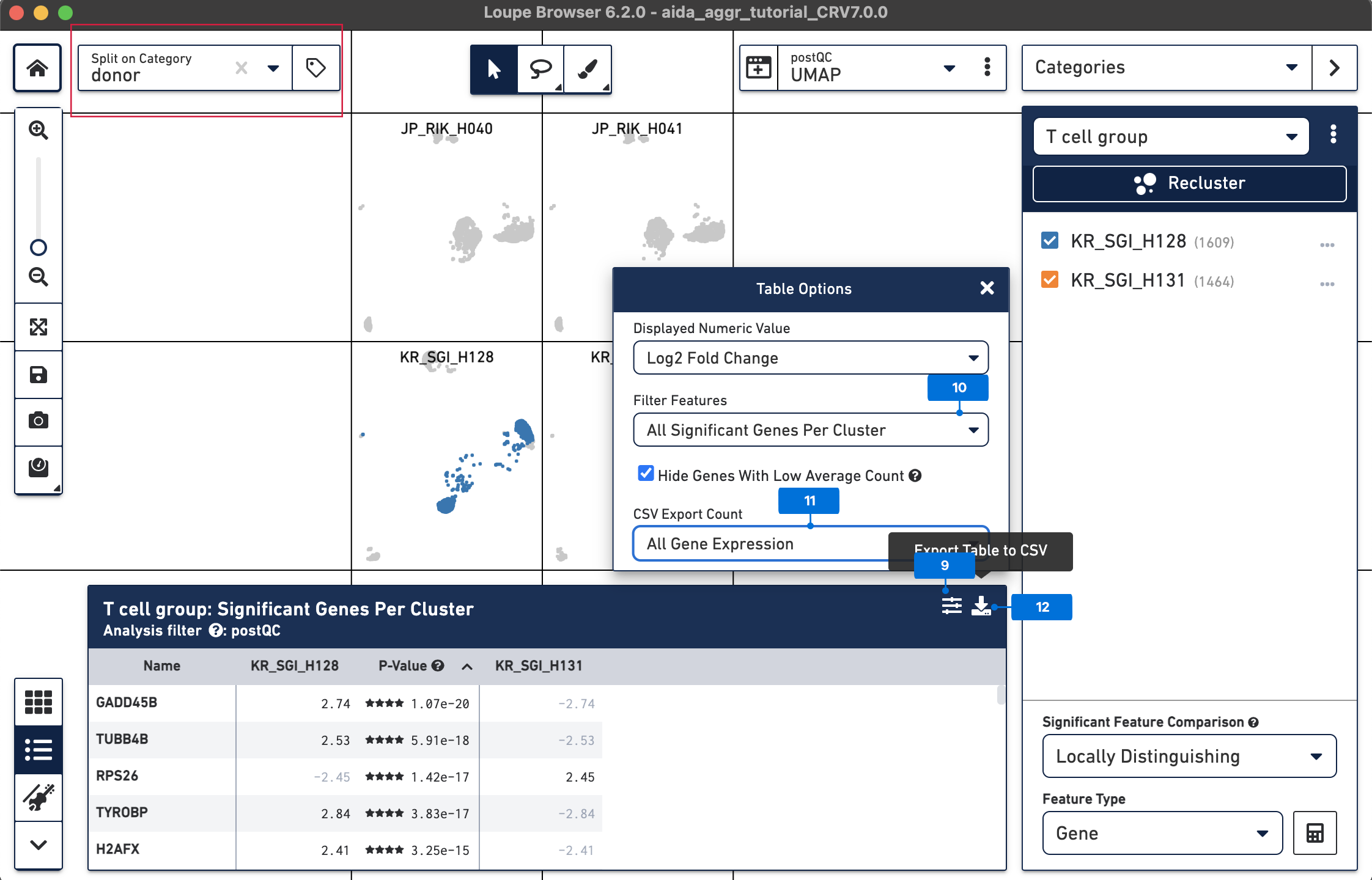
After DEG calling, the results are displayed in the feature table. The DEG table can be exported as a CSV file. 9) Click the Feature Table Options button 10) Select All Significant Genes Per Cluster for Filter Features 11) Select All Gene Expression for CSV Export Count 12) Click the Export Table to CSV button
The DEG list can be used for downstream gene ontology and pathway analyses using third-party tools. The top pathways associated with the significantly up-regulated genes in KG_SGI_H128 (DAVID, log2 fold change>1 and adjusted p-value<0.05) include "Apoptosis" and "Graft-versus-host disease".
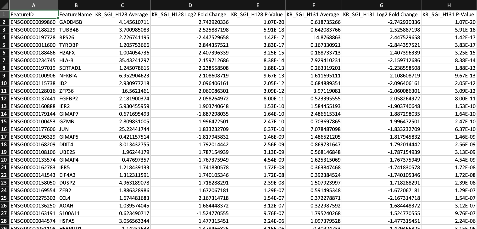
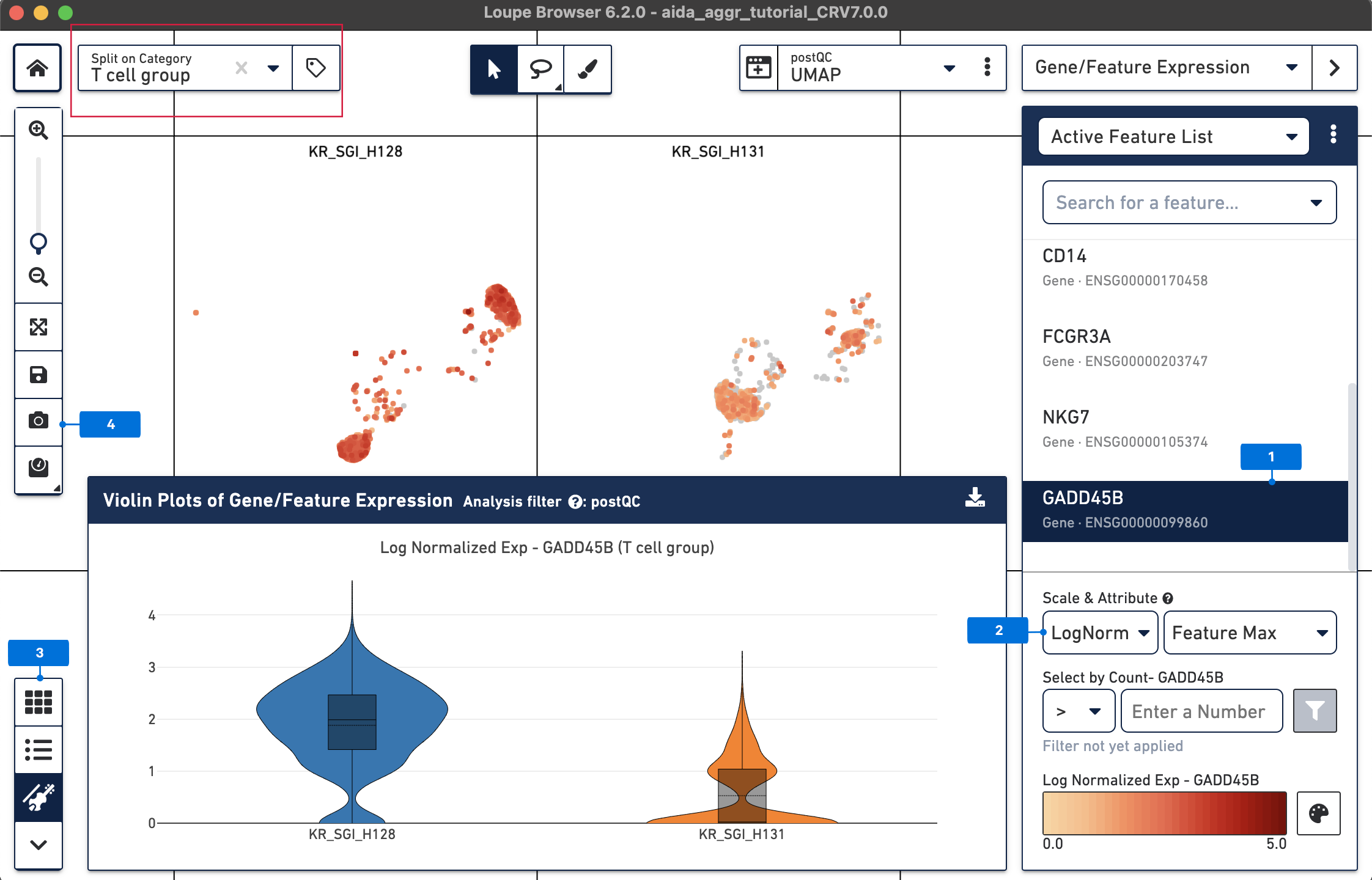
From the above DEG calling, GADD45B is one of the up-regulated genes in T cells from KR_SGI_H128 compared to KR_SGI_H131. GADD45B is a member of a group of genes that respond to environmental stresses by mediating activation of the p38/JNK pathway.
The expression levels of GADD45B in T cells between these two donors can be visualized in a “T cell group” split view stratified by donors.
More analyses can be performed in Loupe Browser, such as sub-clustering of major cell types into cell subtypes. In addition, third-party tools developed in the single cell community are also very useful to address more advanced data analyses, such as RNA velocity (read more in this Analysis Guide about using third-party tools to perform RNA velocity analysis).
The datasets used in the tutorial are part of the Asian Immune Diversity Atlas (AIDA) project. Raw FASTQ files of eight datasets were downloaded from the Human Cell Atlas data portal. These eight datasets represent four samples from two healthy Japanese donors and two healthy South Korean donors (each sample has two libraries). Two Japanese samples were multiplexed in the same batch and then the multiplexed pool was split into two 10x Genomics reactions/libraries. The same strategy was applied to the two South Korean samples. After downloading the FASTQ files, Cell Ranger v7.0 was used to process the sequencing data. One example command line is shown below for the cellranger count pipeline (replace text in red with path to files):
cellranger count \
        --id=KR_SGI_B010_L001_5GEX_H134 \
        --fastqs=/PATH_TO_raw_data/ \
        --sample=KR_SGI_B010_L001_5GEX_H134 \
        --transcriptome=/PATH_TO_cellranger_reference/refdata-gex-GRCh38-2020-A/ \
        --localcores=8 --localmem=64
After running cellranger count on each of the eight datasets (each dataset is from a different GEM well), the cellranger aggr pipeline was used to aggregate them:
cellranger aggr \
        --id=aida_aggr \
        --csv=/PATH_TO_aggregation_csv/sample.csv \
        --localcores=16 \
        --localmem=128
The aggregation CSV file, sample.csv, should contain the following:
sample_id,molecule_h5
JP_RIK_B003_L001_5GEX_H040,path/to/molecule_info.h5
JP_RIK_B003_L002_5GEX_H040,path/to/molecule_info.h5
JP_RIK_B003_L001_5GEX_H041,path/to/molecule_info.h5
JP_RIK_B003_L002_5GEX_H041,path/to/molecule_info.h5
KR_SGI_B010_L001_5GEX_H128,path/to/molecule_info.h5
KR_SGI_B010_L002_5GEX_H128,path/to/molecule_info.h5
KR_SGI_B010_L001_5GEX_H131,path/to/molecule_info.h5
KR_SGI_B010_L002_5GEX_H131,path/to/molecule_info.h5
The cloupe.cloupe in the aida_aggr/outs/count/ directory is the aggregated cloupe file imported into Loupe Browser used for this tutorial.
Ilicic T, et al. Classification of low quality cells from single-cell RNA-seq data. Genome Biology 17, 2016.
Yamawaki T, et al. Systematic comparison of high-throughput single-cell RNA-seq methods for immune cell profiling. BMC Genomics 22, 2021.