Cell Ranger7.1, printed on 04/06/2025
Neutrophils are the most abundant cell type in human white blood cells (leukocytes). If you have followed our workflow recommendations for processing neutrophils (or other granulocytes) using 10x Genomics Single Cell applications, then neutrophils should be present in your single cell gene expression data. However, neutrophils only express around a few hundred genes (Hay et al. 2018). By default, Cell Ranger may filter out neutrophils in the final results.
This tutorial will demonstrate how to preserve and annotate the neutrophils in your data. For additional discussion, refer to the Neutrophil Analysis in 10x Genomics Single Cell Gene Expression Assays Technical Note.
High-level overview:
To capture neutrophils from 3’ or 5’ Single Cell Gene Expression data, you need to:
--force-cells to include low-UMI barcodes.--include-introns option to accommodate increased intron retention in neutrophils.
Note: This tutorial was written with Cell Ranger v6.1.0 and Loupe Browser v5.1.0. Results may vary slightly with other versions of software. If running this tutorial with Cell Ranger v7.0 or later, --include-introns is set to true by default and does not need to be specified.
|
To begin this tutorial, download and install Loupe Browser (version 5.1 or later). This tutorial will not cover the basics of running Cell Ranger or using Loupe Browser. For general information about Cell Ranger and Loupe Browser software, please see our software support website.
This dataset is generated from whole leukocytes of a healthy donor and prepared with Single Cell 3’ Gene Expression assay. The raw FASTQs and output .cloupe files used in this tutorial can be downloaded here. Although we use 3’ Gene Expression data in this tutorial, all the steps also apply to Single Cell 5’ Gene Expression data.
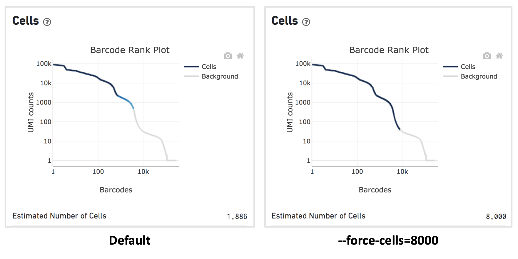
For this dataset, when using the default Cell Ranger cell calling algorithm, there are only 1,886 cells identified (left plot below). This is because the RNA profile of neutrophils is more similar to the background (low UMI, low gene count) and the cell calling algorithm cannot readily distinguish between the neutrophils and background.
Therefore, to capture the neutrophils, we need to override the cell calling algorithm to ensure that low-UMI cells such as neutrophils are included in the filtered feature-barcode matrix. At this stage, there is no need to be concerned about including some background GEMs (Gelbeads-in-Emulsion) to the filtered matrix because we can filter them out later using Loupe Browser or other third-party tools. To override the cell calling algorithm, run cellranger count with the --force-cells option. 10x Genomics recommends starting with the number of cells targeted. If you are unsure about the number of cells expected, it is better to overestimate at this stage.
Given that 8,000 cells are expected to be recovered for this sample, use --force-cells=8000 to analyze this dataset. In the barcode rank plot (right plot below), note a group of lower UMI count barcodes (second ‘knee’) being included as cells, which are likely the neutrophils of interest.
In addition, we also recommend running Cell Ranger with the --include-introns option, which enables Cell Ranger to count reads that map to intronic regions. As neutrophils retain a large number of introns (Ulrich & Guigo, 2020), mapping intronic reads improves the gene sensitivity, which may be useful when analyzing subpopulations.
Given that these are human samples, we will use the pre-built human reference (refdata-gex-GRCh38-2020-A). After determining the path to the reference folder and FASTQ files, run cellranger count:
cellranger count --id=mysample \
--transcriptome=/path/to/refdata-gex-GRCh38-2020-A \
--fastqs=/path/to/fastqs --sample=mysample \
--force-cells=8000 --include-introns
After the pipeline completes successfully, find the .cloupe file in the output directory. Alternatively, download the cloupe.cloupe file for this example dataset. Load this file into the Loupe Browser for cell-type annotation and data filtering.
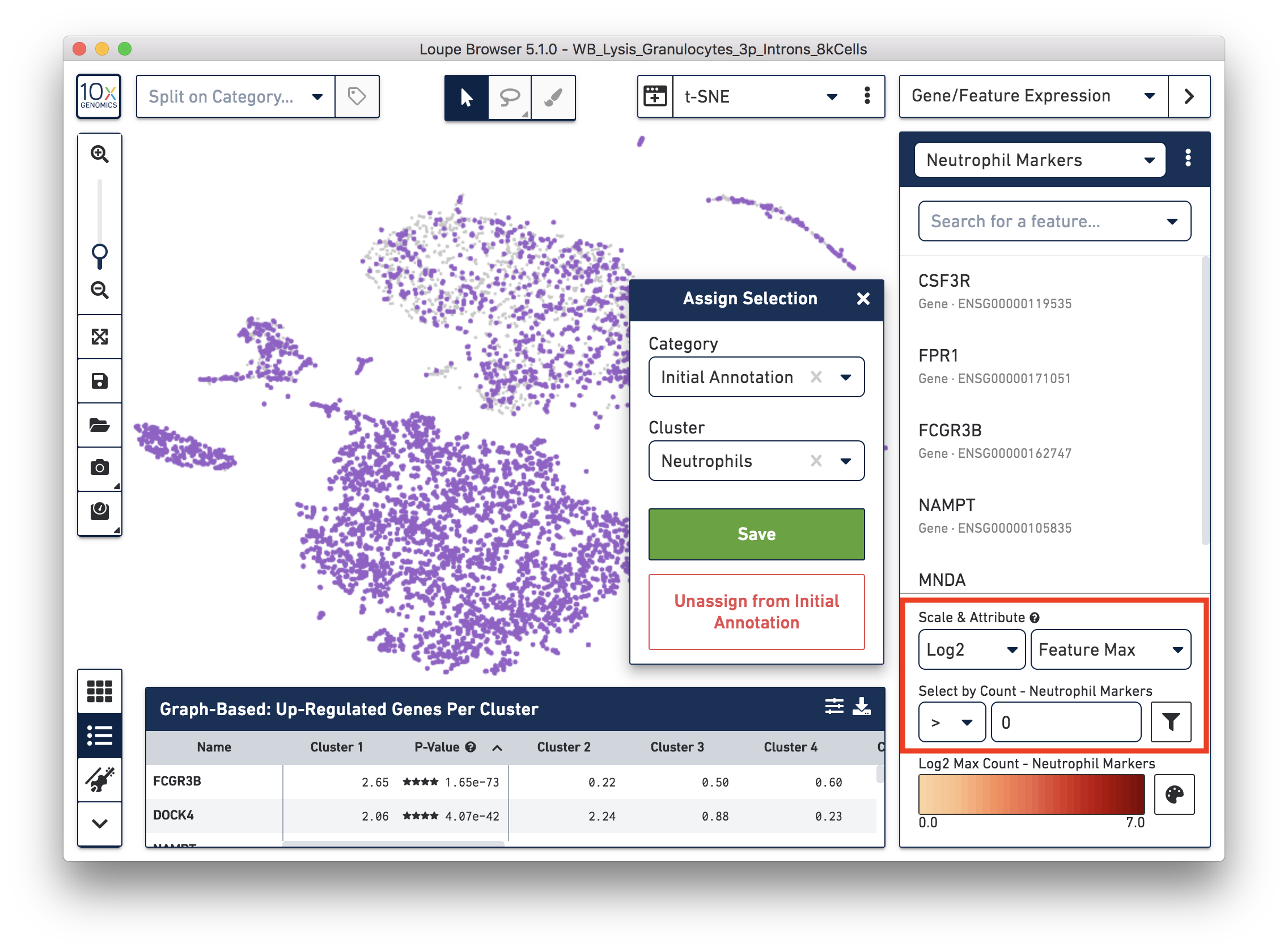
To annotate known cell types, we will use cell markers - neutrophils, B cells, T cells, and monocytes - from this file: BloodCell.csv. These cell markers are selected from the literature and designed for blood samples. If you prefer using other blood cell markers, you can make your own cell marker CSV files. To import the CSV file, in the ‘Gene/Feature Expression’ view, click on the three dots to the right of the ‘Active Feature List’, then select 'Import Lists' from the dropdown menu. Select the CSV file. After import, you should be able to choose the different cell types from the feature list selector.
First, annotate the neutrophils. To select the potential neutrophils, use all the genes in the ‘Neutrophil Markers’ list and set ‘Scale & Attribute’ as ’Feature Max’ > 0. This means that barcodes that express (UMI>0) any neutrophil genes are defined as potential neutrophils. This is a relatively comprehensive marker list, and some of the genes may also be expressed in other blood cell types. In this tutorial, we first select this more extensive group of potential neutrophils and then refine it later.
Next, annotate other cell types. For example, with the monocyte marker (CD14), observe a cluster of monocytes on the t-SNE plot. Select these barcodes with the polygonal selection tool.
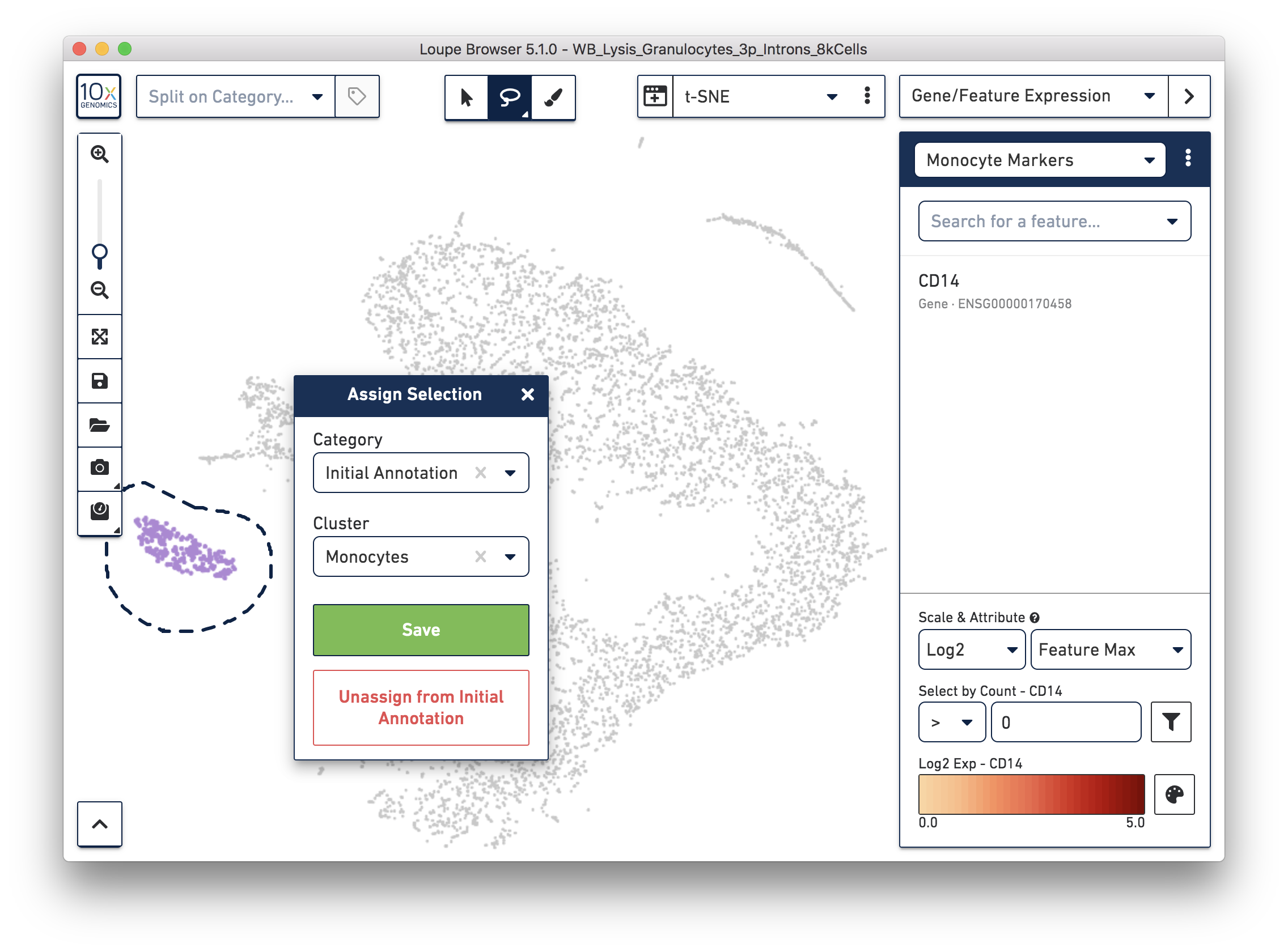
Similarly, you can annotate the B cells and T cells with marker genes and the polygonal selection tool.
After annotating these four major blood cell types, assign the remaining barcodes into the last cluster. You can label them 'Background' for now, given that many of these barcodes are probably background noise.
After annotating the barcodes, we can now use the interactive filtering and reclustering workflow (implemented in Loupe Browser 5.0 and later, see tutorial) to filter out the background GEMs and perform reclustering.
For simplicity, we will only use the ‘Threshold by Features’ and ‘Mitochondrial UMIs’ filters for this tutorial. You could implement the other steps when running your own data.
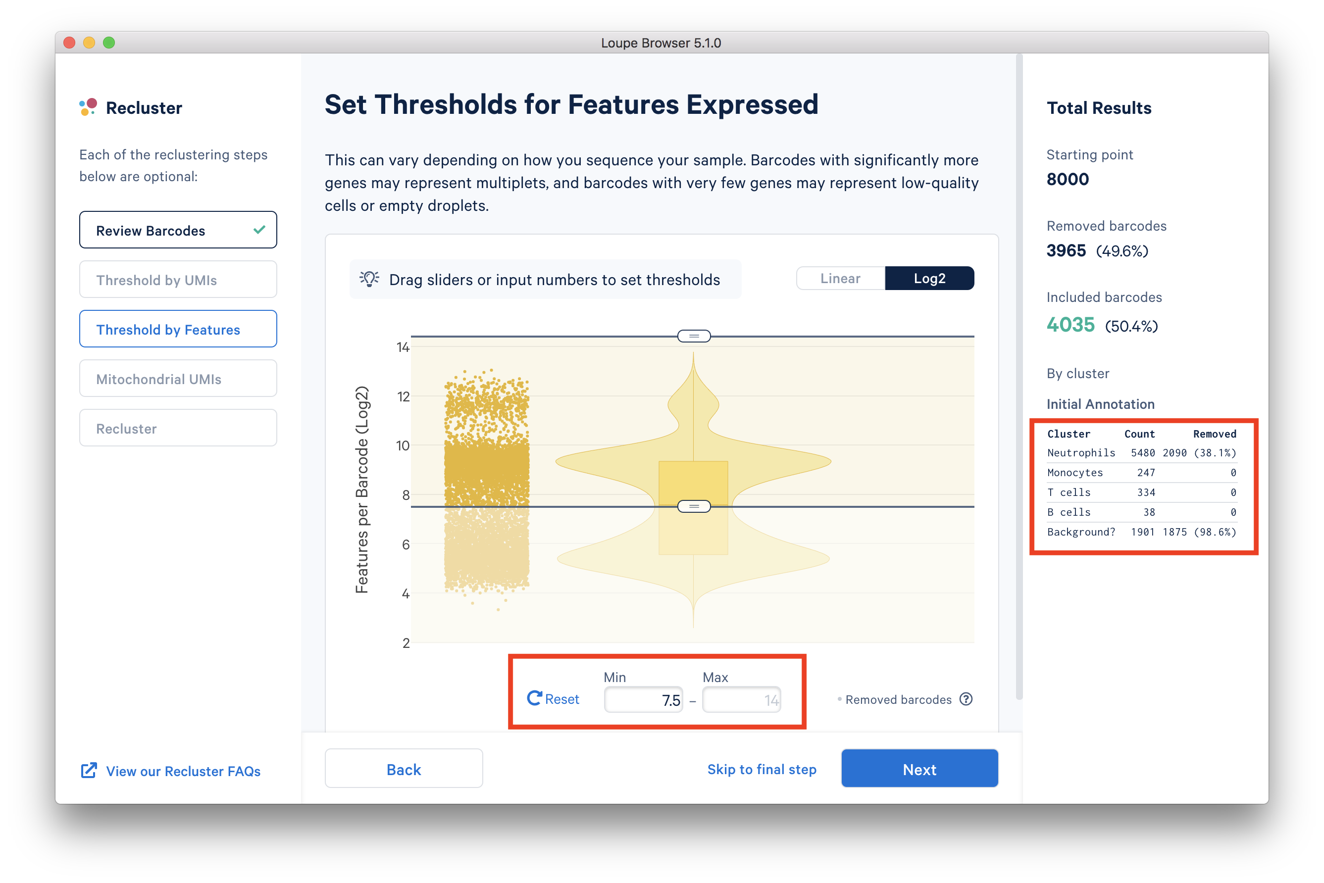
In the ‘Threshold by Features’ step, the ‘Log2’ view shows a violin plot with the number of distinct genes found for each barcode. For this dataset, the violin plot reveals three separate groups of barcodes: The first group has higher numbers of features (genes) detected, mostly B cells, T cells, and monocytes. The group in the middle could be neutrophils because neutrophils are known to only express a small number of genes. The group with the lowest gene counts are likely empty droplets. Given that we forced Cell Ranger to call a very high number of cells, it is expected to have empty droplets in the results.
You can drag the lower slider to somewhere in between the middle and lowest groups, the minimum (Min) value will change as you drag the slider. For example, in this dataset, set the Min to 7.5 in Log2 scale. This value may vary for different datasets, for example, the suitable Min for this example 5’ Gene Expression dataset is 6.
The 'Annotation' box on the right reveals that by setting this threshold, the majority (> 98%) of the empty droplets are removed, but < 40% of the tentative neutrophils are removed.
After setting the 'Threshold by Features' in the Loupe Recluster window, use the ‘Mitochondrial UMIs’ filter to remove poor quality or dying cells. Try using 15% as the maximum threshold, which removes a small number (16) of unhealthy cells. This threshold may also vary depending on the datasets.
When finishing setting the threshold, click the 'Next' to select the type of plot(s) to generate and name the filtered dataset. In this tutorial, we will use UMAP projection due to shorter run time and more clear separation of different cell types. Name it as 'Filtered' and then click 'Recluster' to run the analysis.
Running reclustering may take a few minutes, depending on your computer's specifications. Upon completion, the window will show 'Success'. After clicking 'Done', you will be directed back to Loupe Browser to view the new 'Filtered' category.
Using the reclustered results, you can refine cell type annotation, similar to step 4 above. You can annotate major cell types (neutrophils, B cells, T cells, and monocytes) using the same set of markers in this file mentioned above (BloodCell.csv).
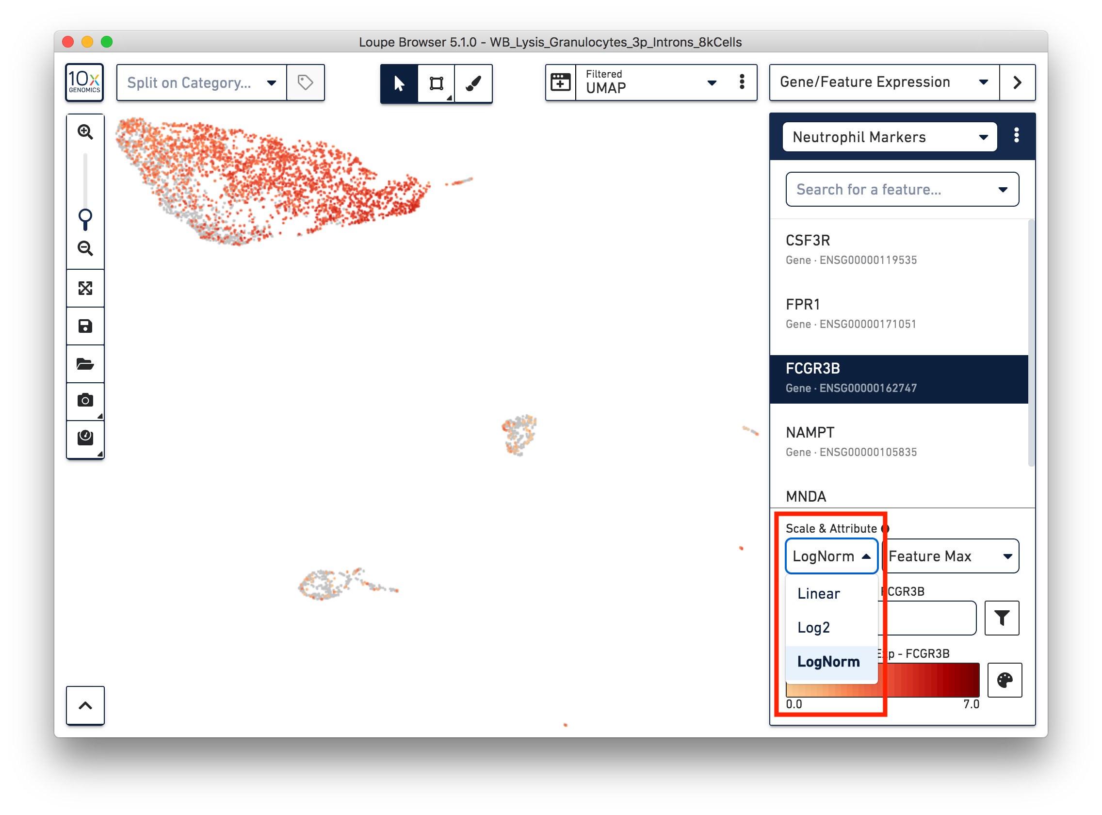
First, refine our annotation of the neutrophils. Given that some of the neutrophil markers are also expressed in other immune cells, it could be useful to view the ‘LogNorm’ value (UMI normalized by total UMI associated with the barcode) of individual marker genes to identify which groups of cells are neutrophils. For example, the profile of FCGR3B expression indicates that the large group of cells at the upper left-hand corner are neutrophils. Therefore, we can select these cells and annotate them as neutrophils.
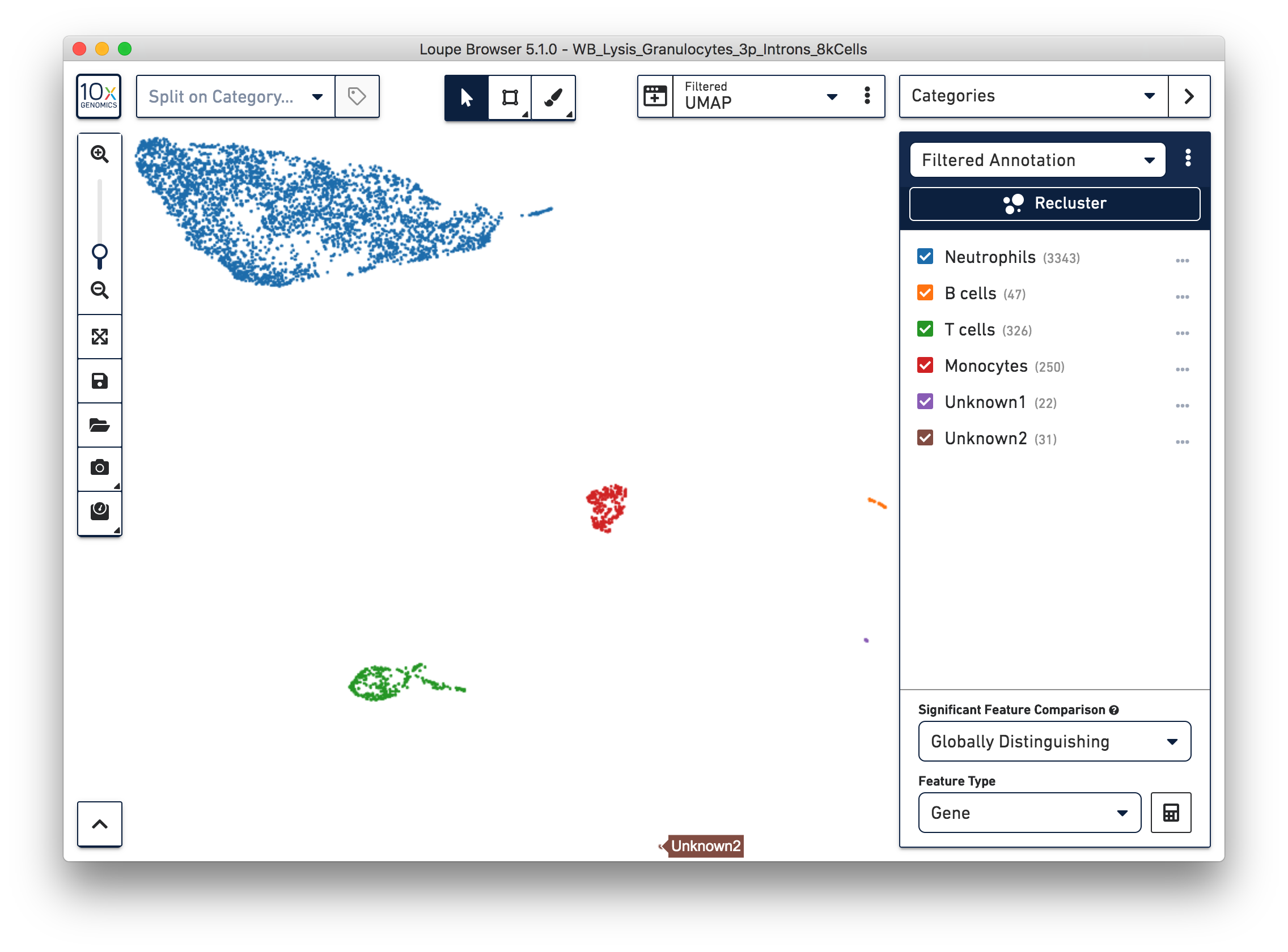
Similarly, we can annotate the B cells, T cells, and monocytes with the marker genes in the CSV file. After annotating the above four cell types, there are still two small clusters of cells, which you can temporarily label as ‘Unknown1’ and ‘Unknown2’.
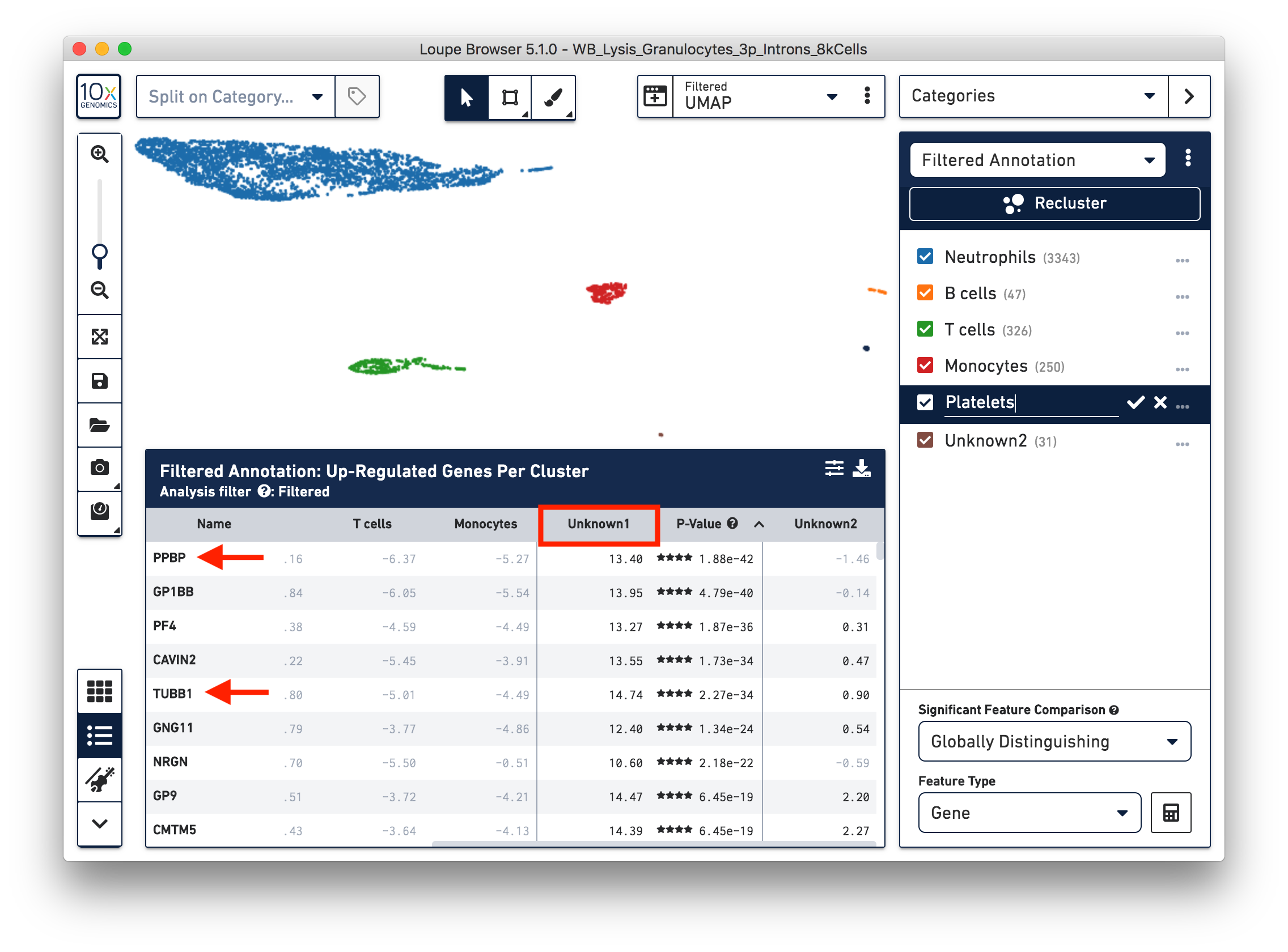
To further annotate the unknown clusters, run a differential expression analysis. The results revealed that the top up-regulated genes for ‘Unknown1’ are PPBP and TUBB1, which are platelet marker genes. Therefore, rename the cluster ‘Unknown1’ as ‘Platelets’.
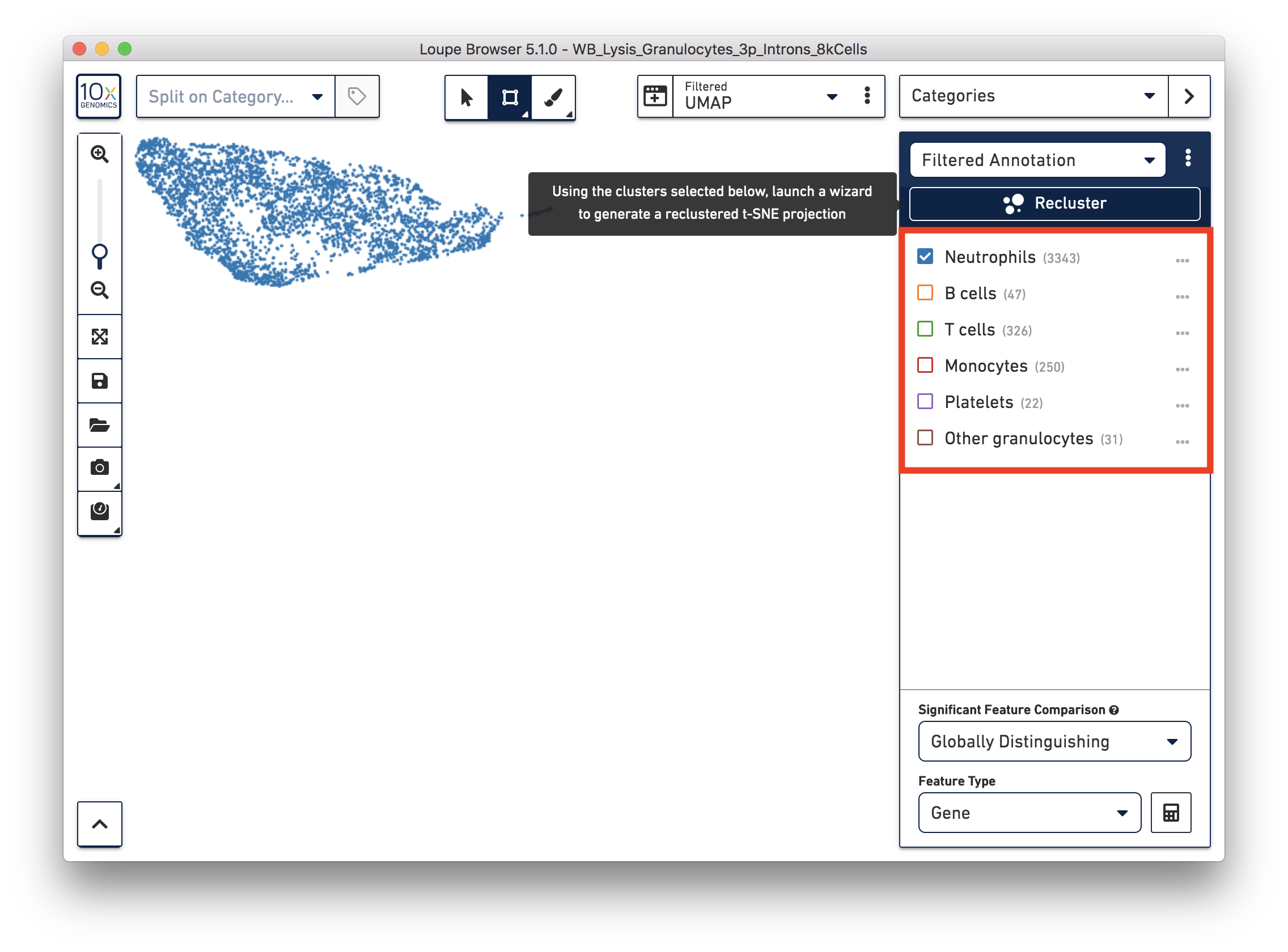
The top up-regulated genes for the ‘Unknown2’ cluster includes HDC, CLC, and IL3RA, indicating that these are other granulocytes (eosinophils or basophils).
All the steps mentioned above also apply to 5’ Gene Expression data. Cell Ranger output from the 5’ data can be found here.
You identified 3,343 neutrophils in the earlier step. If you are interested in neutrophil subtypes, you can run the reclustering again on these neutrophils. To run reclustering on only neutrophils, you can uncheck all the other cell types and then run Recluster.
In the reclustering workflow, you can directly 'Skip to final step’, name it ‘Neutrophils Recluster’, and click ‘Recluster’ to run analysis on only the 3,343 neutrophils.
To explore the substructure of the neutrophil subtypes, you can run a differential expression analysis on the Neutrophils Recluster results. You can further annotate each cluster by checking the top differentially expressed genes. For example, the cells at the bottom of the UMAP (Cluster 4) are enriched for some marker genes (LTF, S100A12) of neutrophil early maturation (Combes et al. 2021).
Furthermore, you can load the data to third-party tools for additional analysis. In this case, we used scVelo (Bergen et al. 2020) to infer the dynamics involved in neutrophil maturation. We projected the maturation dynamics and latent time (represents the biological process) in the UMAP.
This analysis identifies transitions starting in Cluster 4 and ending in Cluster 2. This is also represented by the latent time values in each of the different subpopulations. Finally, we inspected the expression of genes previously described in neutrophil maturation (Combes et al. 2021) and observed transcriptional dynamics following the previously described transitions.
For additional detail on how to perform the analysis illustrated in the figure above, please refer to this Analysis Guide tutorial: Trajectory Analysis using 10x Genomics Single Cell Gene Expression Data. Note: 10x Genomics does not provide support for community-developed tools and makes no guarantees regarding their function or performance. Please contact tool developers with any questions. If you have feedback about Analysis Guides, please email analysis-guides@10xgenomics.com.
The example dataset we used in this tutorial showed clear separation between neutrophils and background GEMs (shown in step 5 above). For some other datasets, there might not be a clear separation between them. One possibility is that the neutrophils in the sample were not in good condition, and their profiles are indeed more similar to empty droplets.
If you have determined that there is no workflow issue and would still like to detect the neutrophils, you can analyze the marker genes and clustering results. In the example below, we can see a group of cells (in red) has higher expression of neutrophil markers, such as NAMPT.
These cells are in ‘Cluster 6’ from Graph-Based clustering. You could also check the top differentially expressed genes in the Feature Table. For datasets with large amounts of neutrophils, it might be necessary to uncheck the ‘Hide Genes With Low Average Count’ option. This is because of the overall low gene expression levels in neutrophils.
Therefore, for this dataset, although we cannot observe a clear separation between neutrophils and background based on UMI or feature counts (data not shown), we could still use clustering results and marker genes to identify neutrophils. The underlying rationale is that neutrophils may have similar total UMI counts as background, but the overall gene expression profile is distinct from the background. Alternatively, you could try using third-party tools (for example, CellBender) to separate the neutrophils from the background.
Bergen V, et al. Generalizing RNA velocity to transient cell states through dynamical modeling. Nature Biotechnology 38: 1408-1414, 2020.
Combes A, et al. Global absence and targeting of protective immune states in severe COVID-19. Nature 591: 124-130, 2021.
Hay S, et al. The Human Cell Atlas bone marrow single-cell interactive web portal. Experimental Hematology 68: 51-61, 2018.
Ullrich S and Guigo R. Dynamic changes in intron retention are tightly associated with regulation of splicing factors and proliferative activity during B-cell development. Nucleic Acids Research 48: 1327-1340, 2020.