Space Ranger6.1, printed on 03/10/2025
Goal: To find subgroups within the clusters and perform differential gene expression.
This tutorial will showcase how to isolate subclusters and identify key differentiating gene markers using a preloaded mouse brain dataset in Loupe Browser.
In addition to projecting the spots and their associated clusters onto the image, the clustering can also be viewed as a t-SNE or UMAP projection. The linked window option ![]() allows you to visualize both views simultaneously.
allows you to visualize both views simultaneously.
In this example, the UMAP projection is chosen in the main window using the view selector. Click ![]() and select Spatial to open the image view in a new window. Note that the clusters colors have been updated from default. Refer to Spatial Clusters tutorial to learn more.
and select Spatial to open the image view in a new window. Note that the clusters colors have been updated from default. Refer to Spatial Clusters tutorial to learn more.
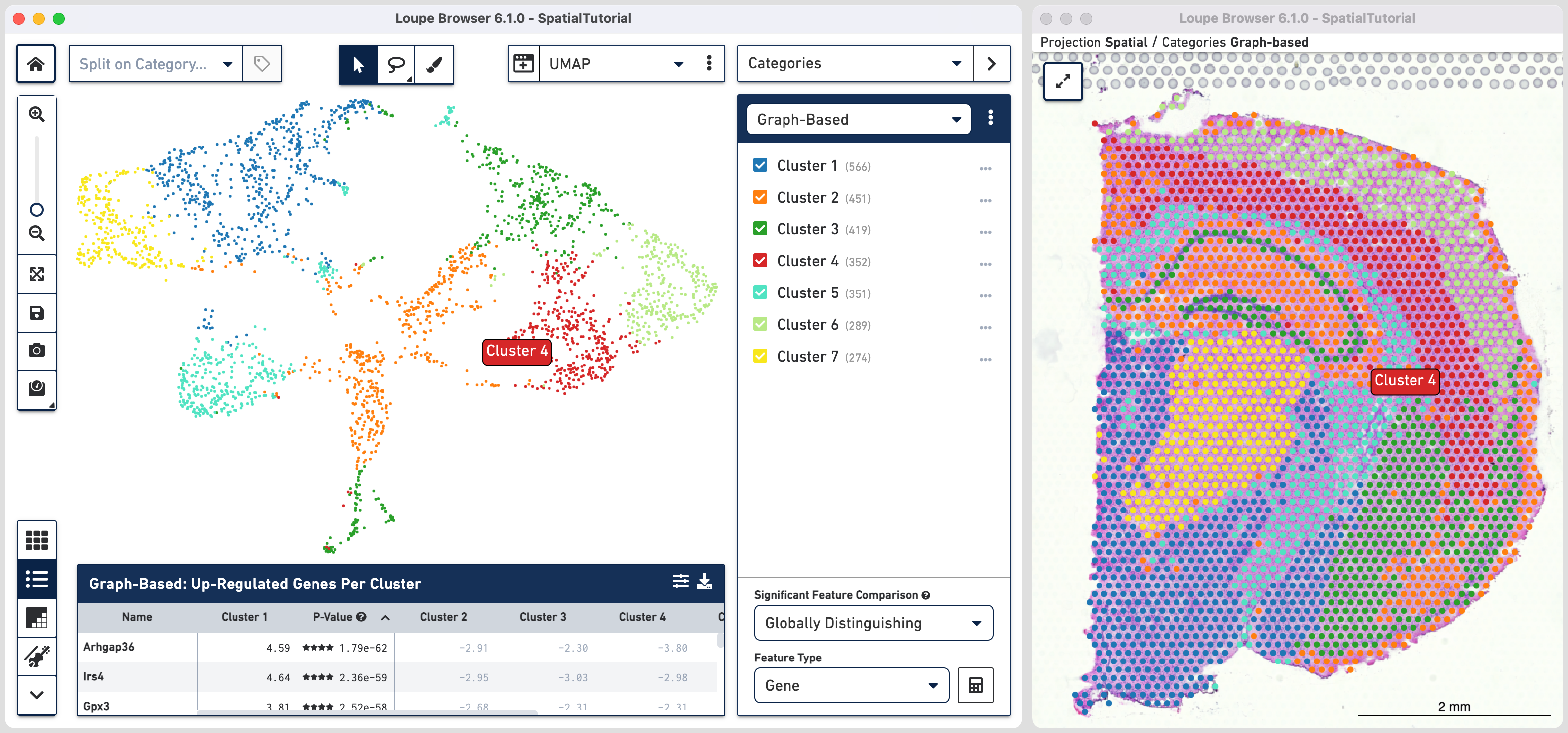
The default clustering results used in this view are from the Graph-based
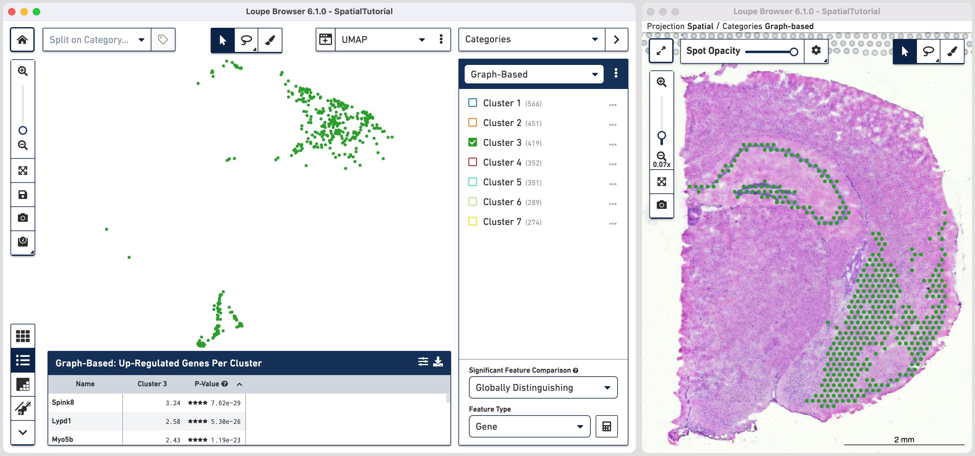
clustering method. The size of the spots can be adjusted using ![]() to make them easier to
see. Unselect the Auto-scale box and move the slider to set the markers to desired size. More details in Toolbox description in the Navigation
tutorial.
to make them easier to
see. Unselect the Auto-scale box and move the slider to set the markers to desired size. More details in Toolbox description in the Navigation
tutorial.
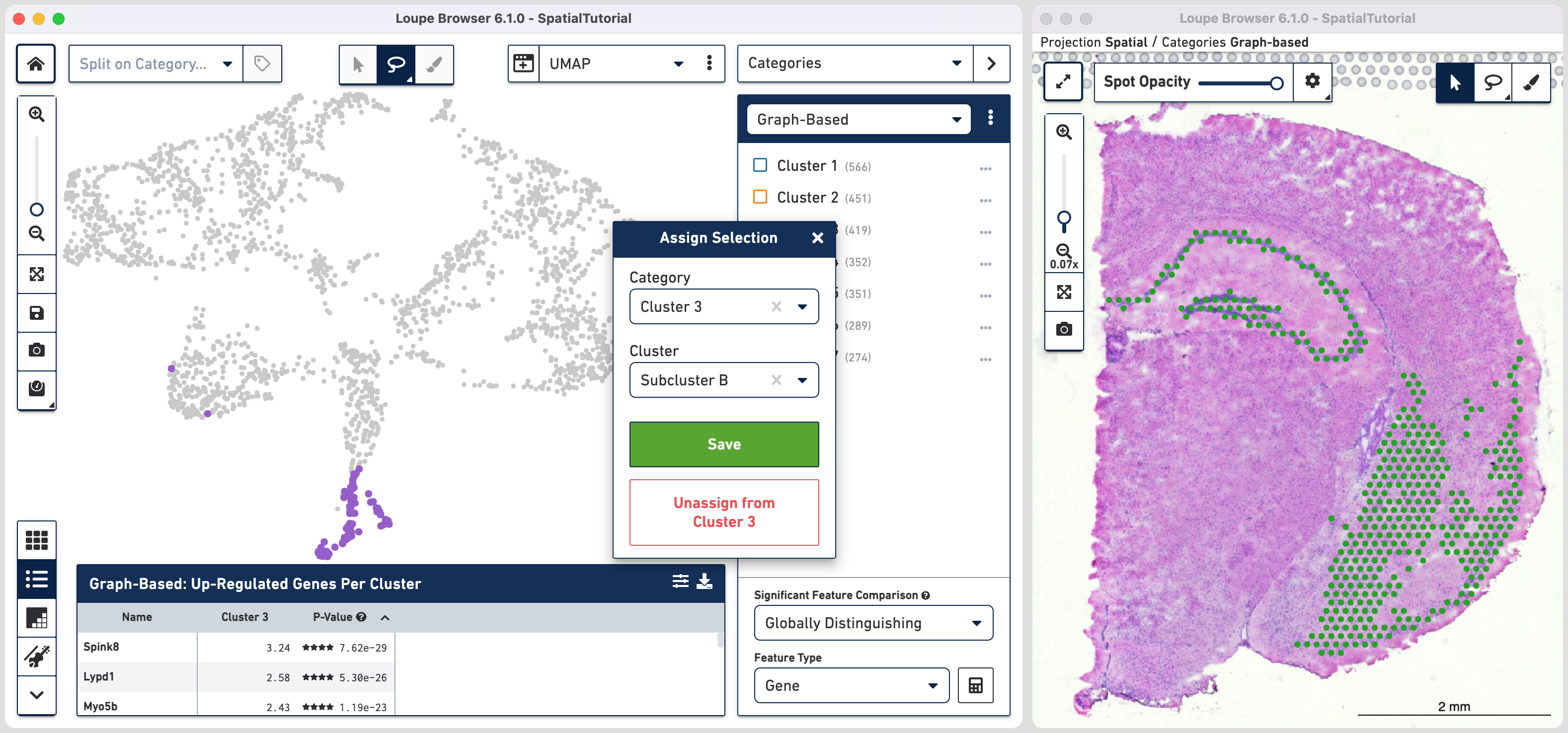
The spots belonging to Cluster 3 on the image are spread over two very different regions in the brain tissue sample. To isolate this, uncheck all of the other clusters.
In order to explore these two subclusters more, create new groups, one for each sub-cluster. To do this, use ![]() to manually select one group of spots, create a new Category called Cluster 3 and a new Cluster name called Subcluster A.
to manually select one group of spots, create a new Category called Cluster 3 and a new Cluster name called Subcluster A.
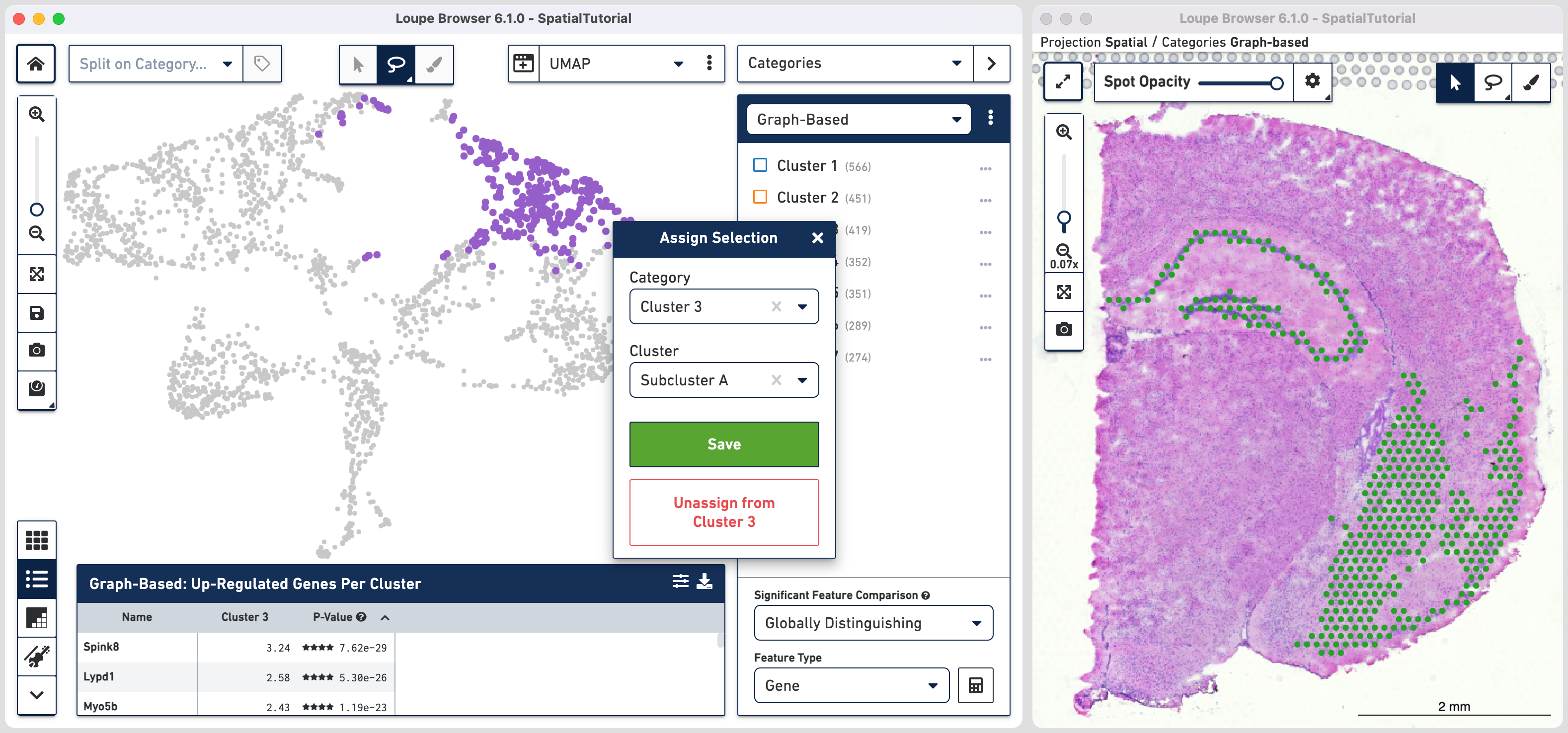
From this Cluster 3 view, go back to the Graph-Based view and repeat the steps to select the second group of spots. Associate the spots to the same Category Cluster 3, but assign them to a new Cluster Subcluster B.
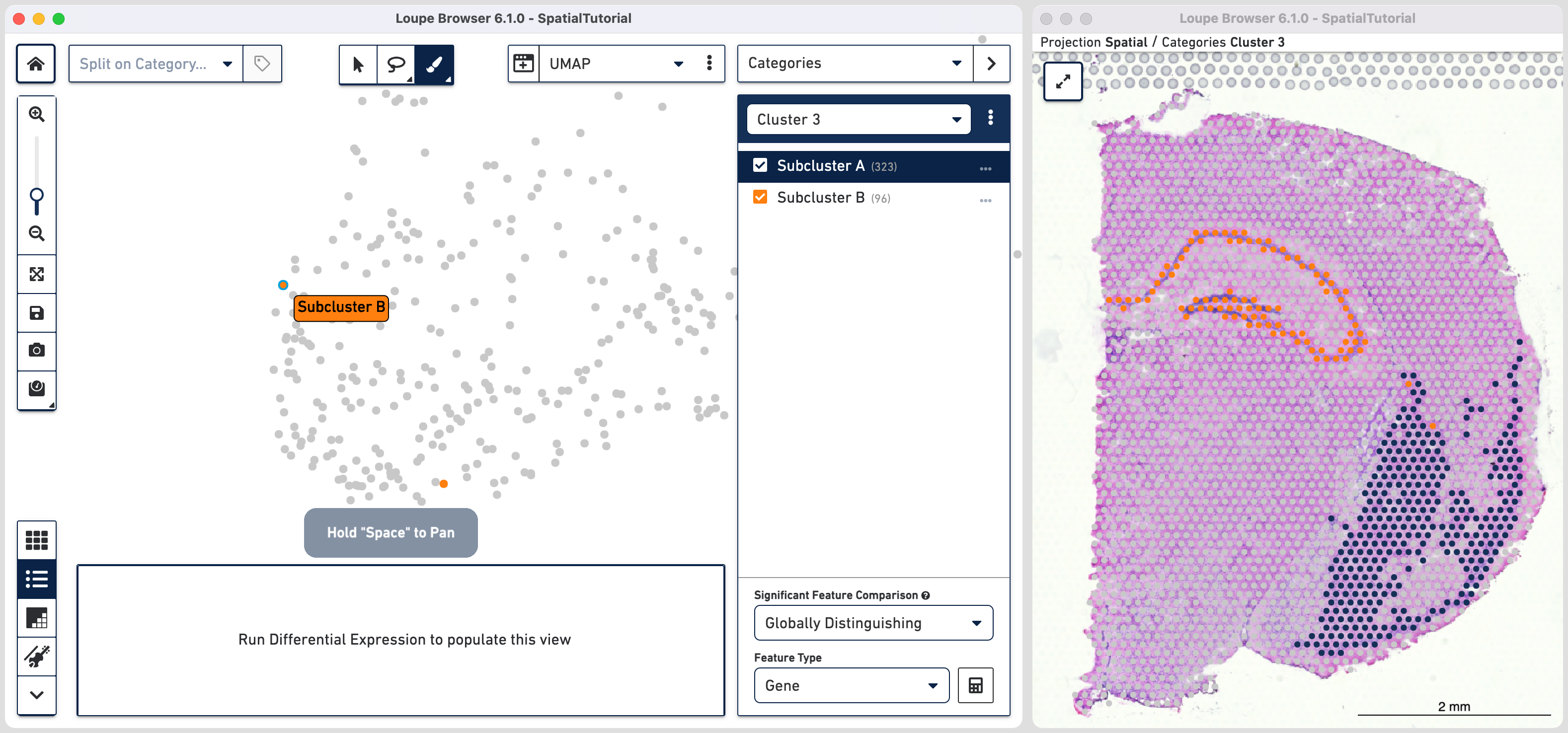
Comparing the projection view for Cluster 3 with the spatial view, there are two spots within the Subcluster A labelled as belonging to Subcluster B. We can correct this by these steps:
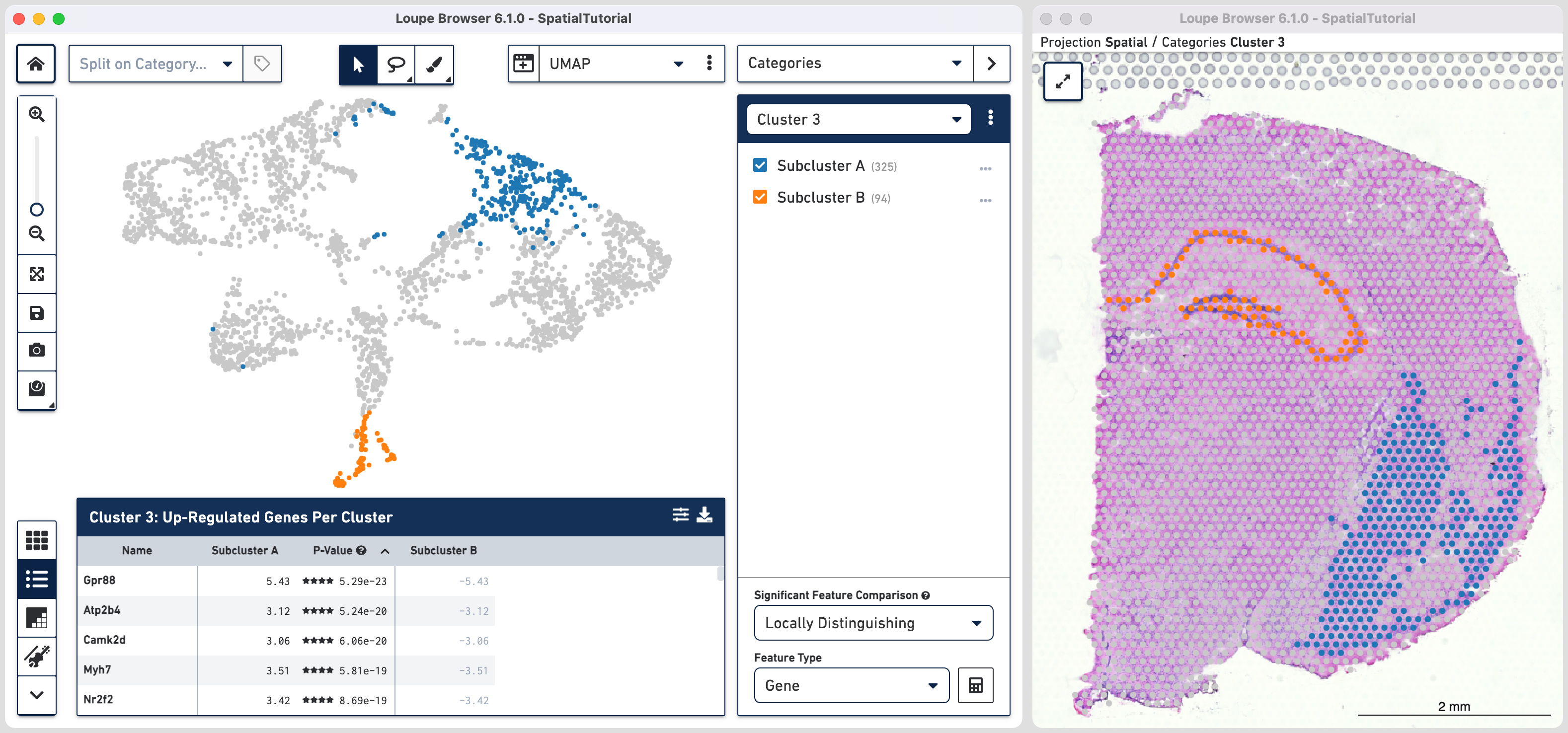
As we are interested in differences between these two Subclusters, choose the Locally Distinguishing option from the
Significant Feature Comparison selector in the bottom right and click calculate![]() . Refer to the computing significant genes to learn more about the this option.
. Refer to the computing significant genes to learn more about the this option.
The data panel view is that of the Feature Table ![]() which by default lists the top differential expressed up-regulated genes. You can change this behavior by clicking
which by default lists the top differential expressed up-regulated genes. You can change this behavior by clicking ![]() to change the Filter Features options. The table can be exported in CSV format by clicking
to change the Filter Features options. The table can be exported in CSV format by clicking![]() .
.
Comparing the top three genes for each cluster, we can confirm that the gene expression corresponds to the spatial distribution of associated cell types.
| Name | Subcluster | Enriched Cells | Matches Spatial Location |
|---|---|---|---|
| Gpr88 | A | D1 and D2 medium spiny neurons in striatum | Yes |
| Atp2b4 | A | Ecitatory neurons in cerebral cortex | Yes |
| Camk2d | A | Excitatory neurons of cerebral cortex and amygdala | Yes |
| Olfml2b | B | Excitatory neurons of CA3 and granule neuroblasts in dentate gyrus | Yes |
| Lefty1 | B | Excitatory neurons of CA1 hippocampus subfield | Yes |
| Lct | B | Excitatory neurons of CA1 and CA3 hippocampus subfields and Granule neurons in dentate gyrus | Yes |
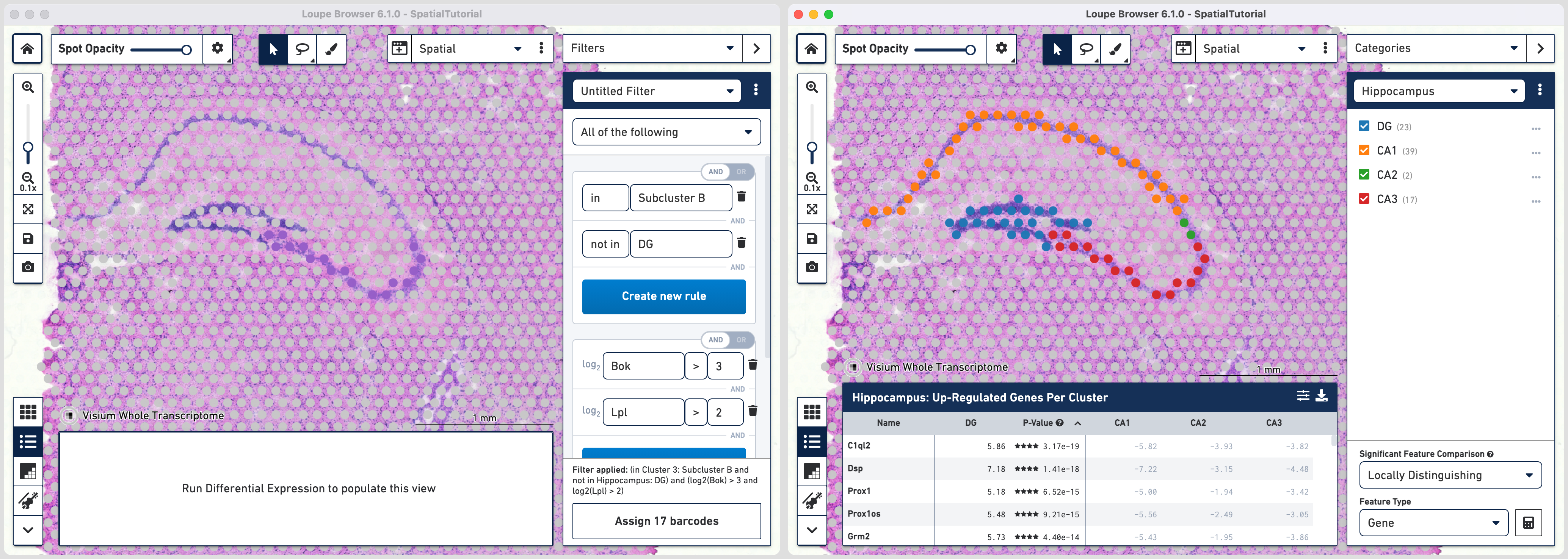
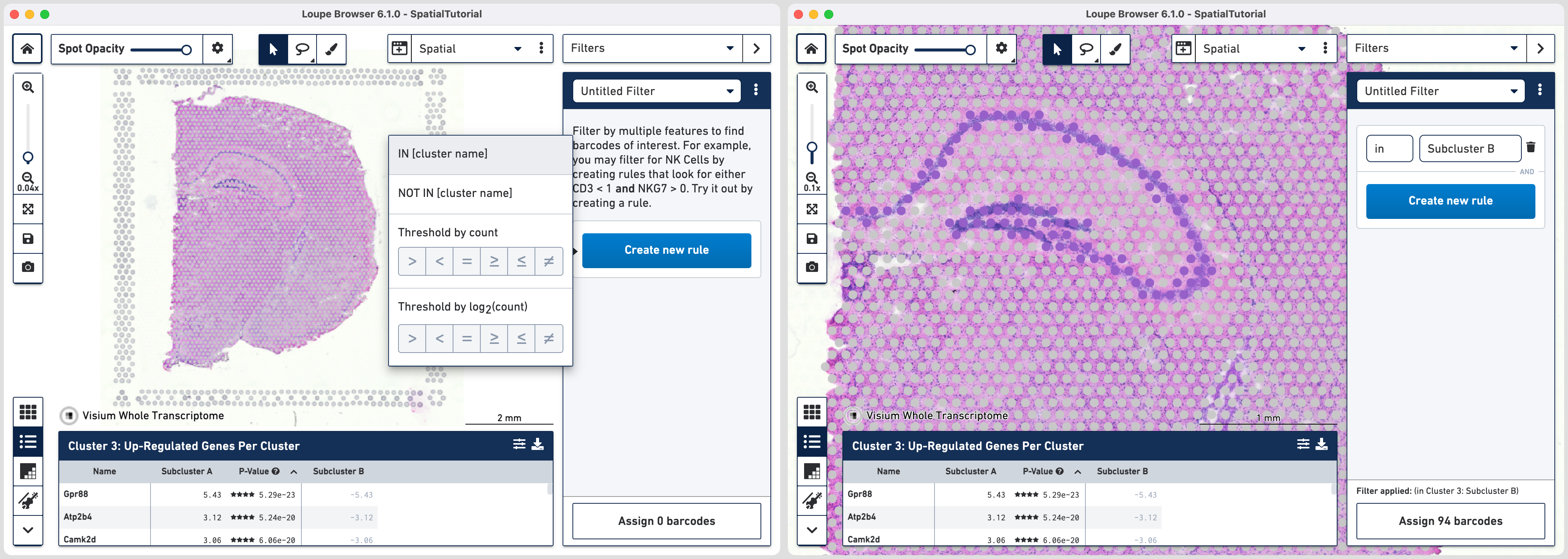
Subcluster B which spatially corresponds to the hippocampus region is made of four distinct subfields. Loupe Browser offers the ability to set up filters to identify barcodes for these subfields. The filtered barcodes from regions of interest can subsequently be exported to be used in community developed analysis tools.
To get started, go back to spatial view in the main window. Click on the mode selector, choose Filters option and click to get started.
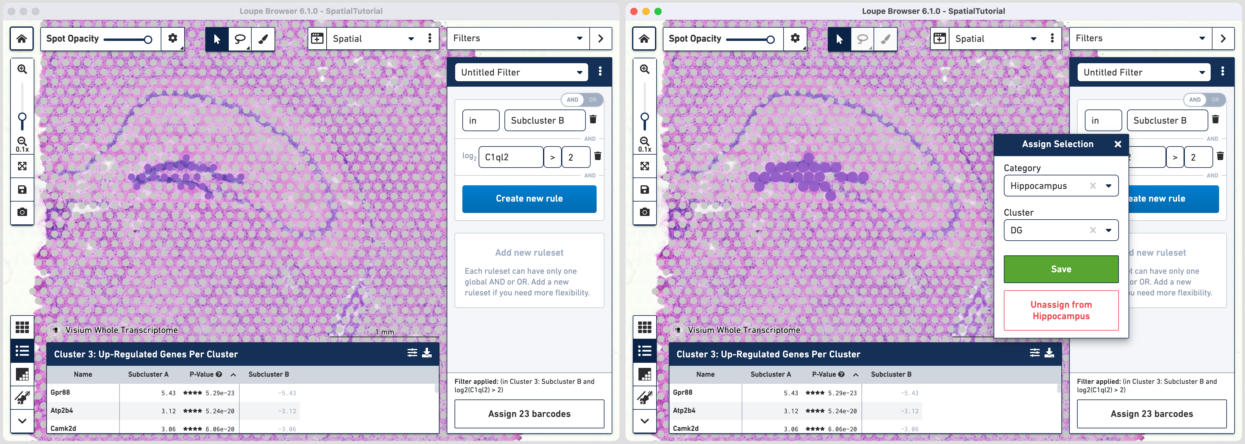
The first rule corresponds to spatial location. Choose IN [cluster name] and input Subcluster B in the Cluster box. All the spots where the filter is applied appears in purple. A human-readable version of the filter is visible at the bottom of the panel along with the number of barcodes eligible after filtering.
Click to add additional rule. The second rule corresponds to identifying the dentate gyrus subfield using log2(count). Choose > under Threshold by log2(count), enter C1ql2 in the feature box and set the threshold at 2.
Click to create a new Category called Hippocampus and a new Cluster called DG.
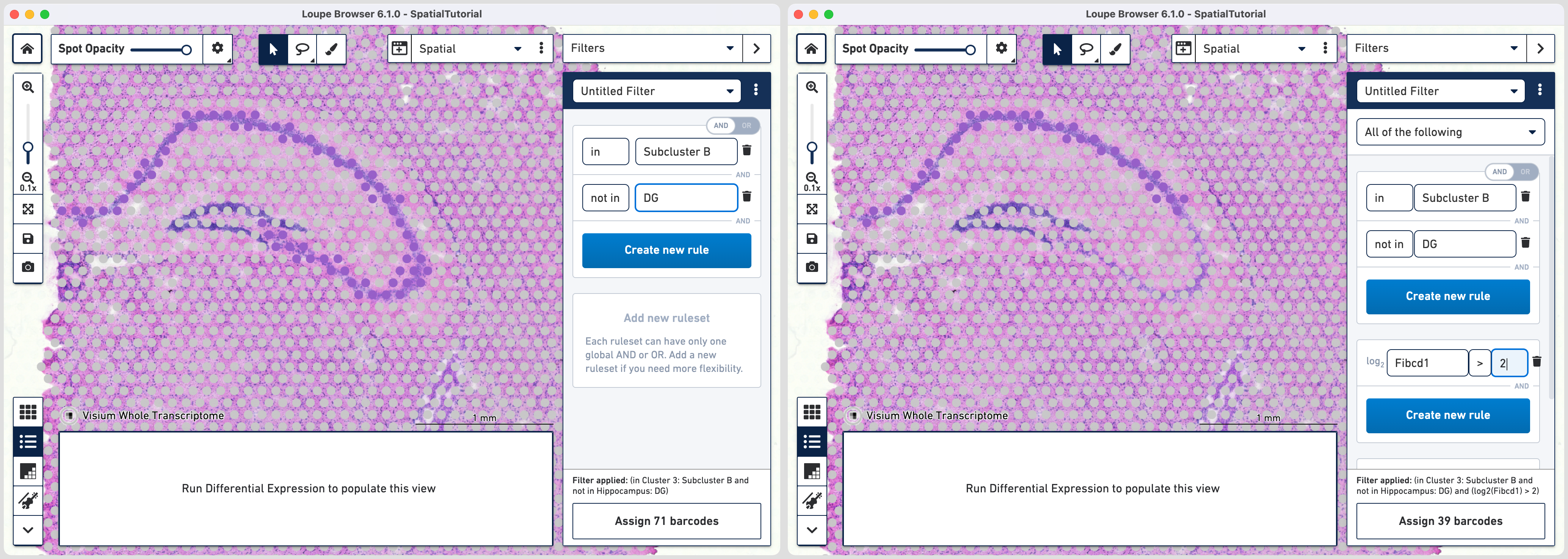
Go back to the Filters mode. The third rule corresponds to CA1 subfield. First, delete the existing filter for DG marker by clicking![]() . Click and choose
. Click and choose NOT IN [cluster name] and select DG from the list. The purple spots are updated to reflect the filter. This rule is the global rule that will apply for all CA subfield selections.
To apply the third rule, click and click .
Choose > under Threshold by log2(count), enter Fibcd1 in the feature box and set the threshold at 2. Click to Hippocampus category and a new Cluster called CA1.
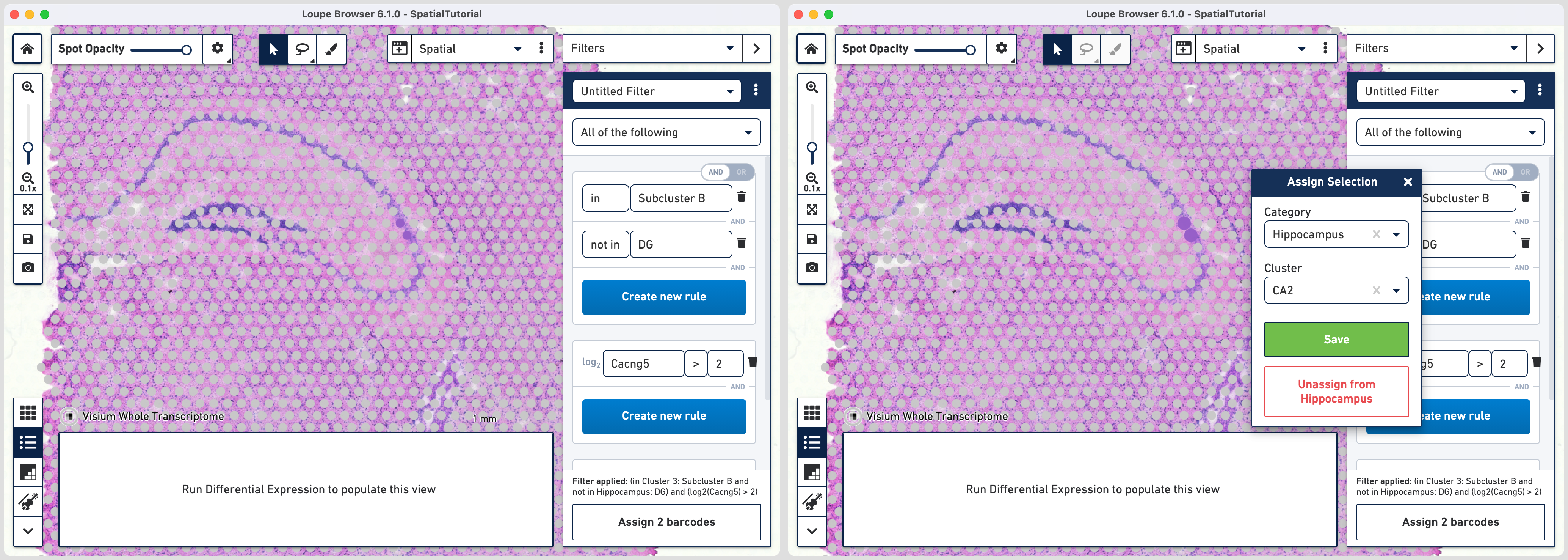
Follow the same steps as those for third rule. Note that since the global rule is already defined, only the subfield specific rule needs to be applied. For the fourth rule, update the second ruleset with Cacng5 with threshold of 2. Assign the filtered barcdoes using to Hippocampus category and a new Cluster called CA2.
For fifth rule, update the second ruleset with Bok with threshold of 3. Click in the second ruleset to add an additional rule.
Choose > under Threshold by log2(count), enter Lpl in the feature box and set the threshold at 3. Note that the AND/OR apply to each ruleset you create offering the flexibility to build complex filters. Assign the filtered barcdoes using to Hippocampus category and a new Cluster called CA3.
With the subfields defined, to analyze the differential gene expression between these regions, choose the Locally Distinguishing option from the Significant Feature Comparison selector in the bottom right and click calculate![]() .
.