Space Ranger6.3, printed on 03/29/2025
The Space Ranger-generated clustering and projection analysis contained in a .cloupe file includes all barcodes from the tissue-associated spots. However, it may be desirable to only analyze a subset of the clusters or subregions of interest, or to remove clusters from the analysis.
Loupe 6.3 introduces an interactive filtering and reclustering workflow for spatial datasets that provides this flexibility. Going through the workflow steps, one can select clusters or regions of interest, filter by UMIs or Features, and compute Louvain graph-based clustering, t-SNE, and UMAP projections.
In this tutorial, the concepts associated with reclustering will be demonstrated by selecting a subset of clusters or subregions in a preloaded mouse brain dataset in Loupe Browser.
The Recluster workflow can be accessed under any of the results in the Categories mode (either Graph-Based, K-Means or manual) by clicking which opens in a new window.
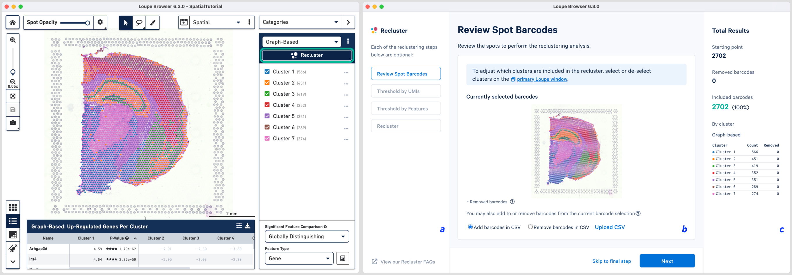
The Recluster window consists of three components: (a) the current workflow step on the left, (b) tooling for the active step in the middle, and (c) statistics about the removed barcodes on the right. To progress through each step, click or choose to skip filtering steps.
The first step allows initial filtering by cluster selection, or a barcode list. The Recluster window is linked to the primary window; by default, all the clusters are selected. Changing either the clustering type (Graph-Based, K-Means or manual), or de-selecting clusters in the primary window, is reflected in the reclustering window.
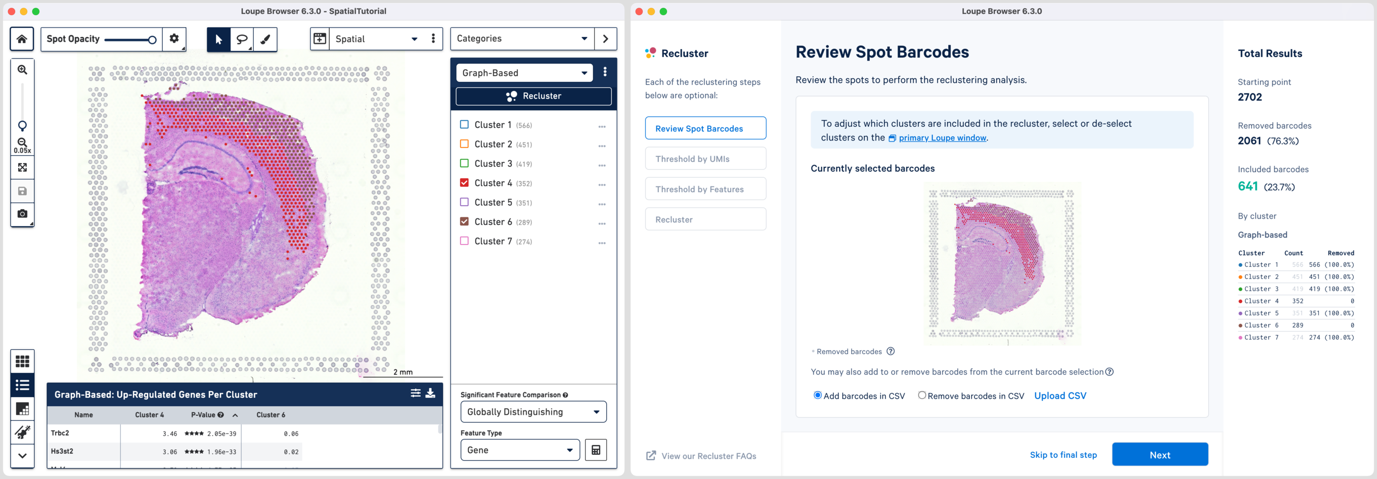
In this tutorial, for the cluster-based selection, clusters 4 and 6 are selected in the primary window. The anatomical region corresponding to these clusters is the isocortex. Subsequently, the reclustering window is automatically updated, listing both the sum total and per-cluster distribution of the included barcodes.
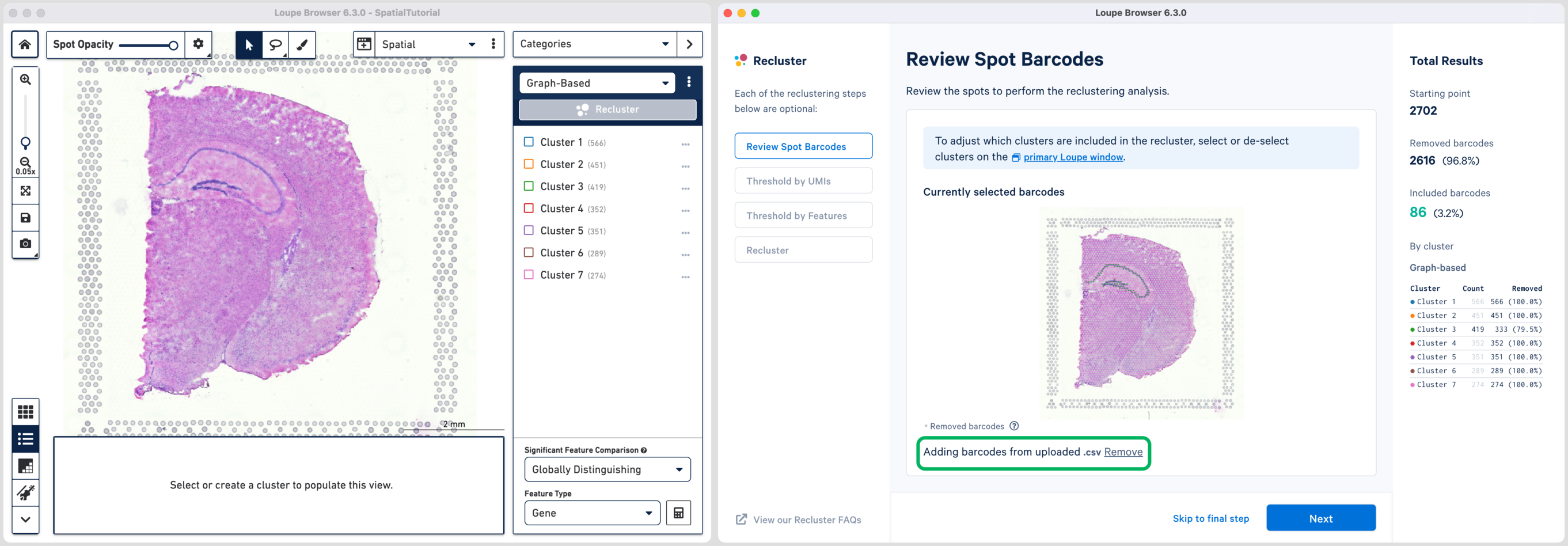
Reclustering can also be applied to custom categories or regions created using Loupe functions such as lasso tools, boolean filters, or CSV list imports. The customizations can be applied in the main window by creating new categories followed by reclustering, or by importing a CSV file directly using the option. For the former option, it is recommended that the custom categories be created prior to initiating the reclustering workflow.
The hippocampus will be used to demonstrate the subregion-based selection. Download a predefined barcode list from the embedded tutorial file. Unselect all the clusters in the primary window and upload the CSV file in the recluster window. Successful upload will update the recluster window to show colored spots tracing the hippocampus on the spatial image.
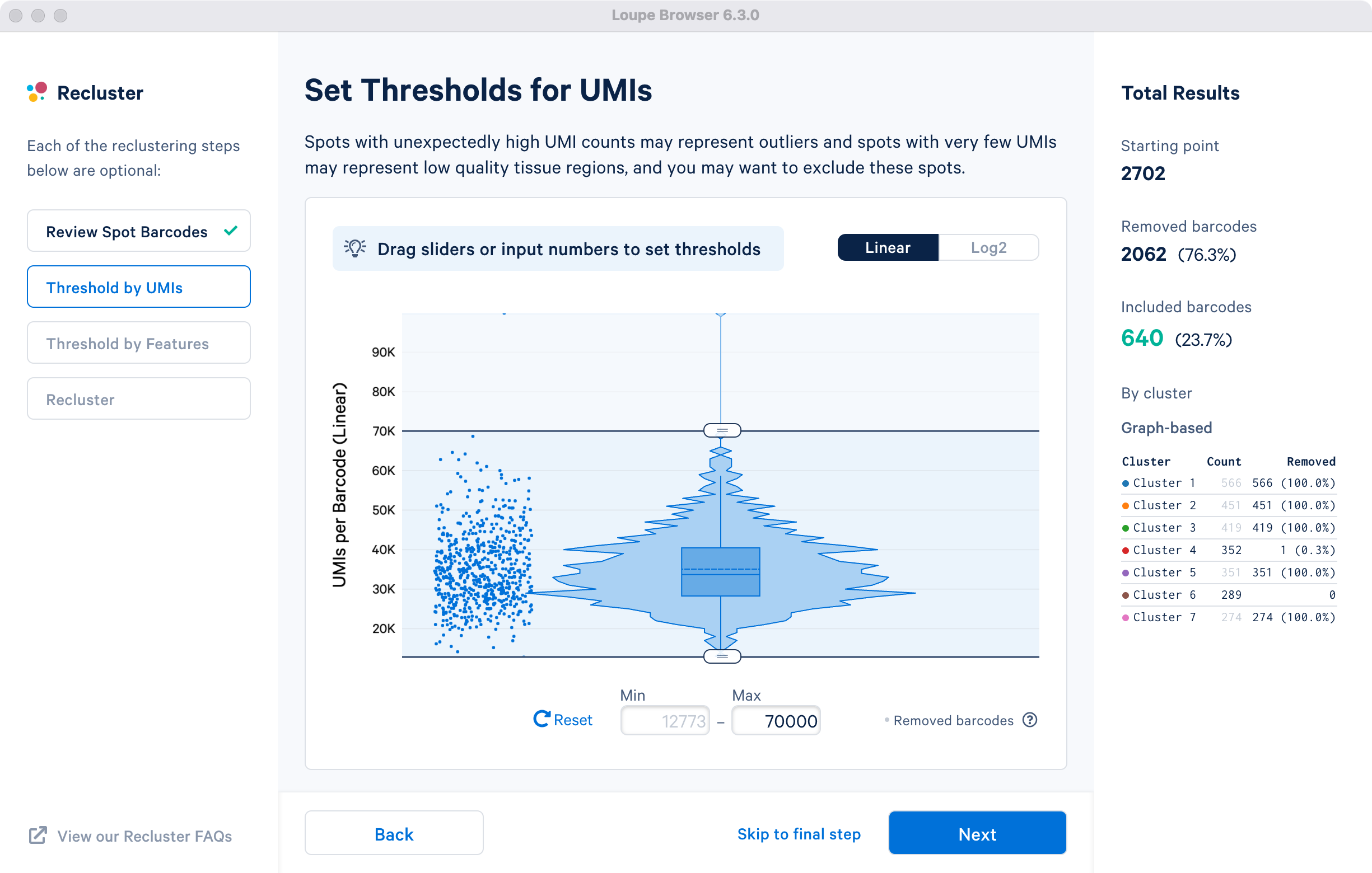
This step allows for filtering by UMI count values for a given barcode or spot for spatial datasets. A violin plot and a box plot of the currently selected barcodes, along with columnar data points for each spot, are shown in the window. By default, the values are shown on linear scale, with an option to view the distribution in log2 scale. Apply the threshold by either moving the sliders on top or bottom of the plot, or by manually entering numeric values in the boxes under the plot.
For demonstration in the cluster-based selection, an upper UMI count limit of 70,000 UMIs per barcode on the linear scale will be used. The statistics on the left are updated to indicate removal of one spot from cluster 4. This filtering step is skipped for the subregion-based selection.
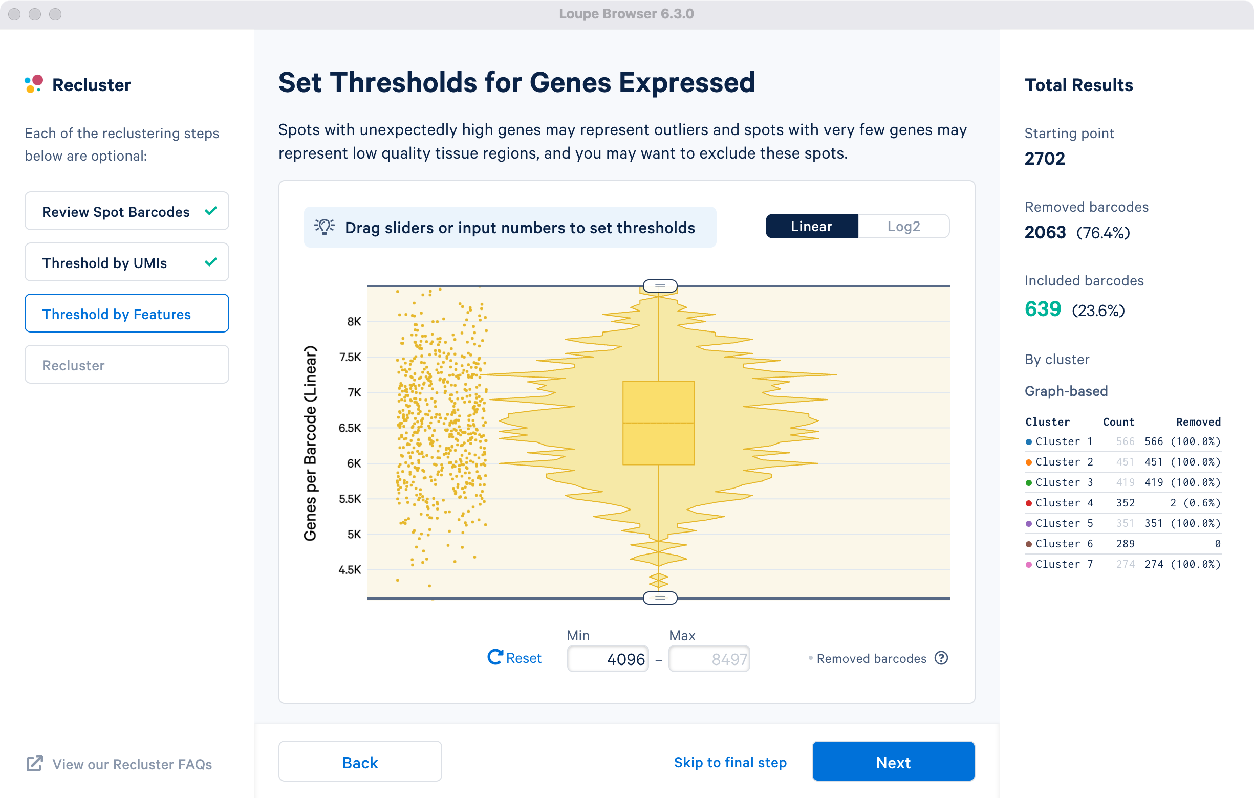
This step allows for filtering by the distinct numbers of detected features i.e. genes per barcode or spot for spatial datasets. Depending on the experiment and tissue type, barcodes with anomalously low or high numbers of distinct features may be undesirable.
For the purpose of this tutorial, in the cluster-based selection example, a lower feature count bound of 4096 features per barcode on the linear scale (12 equivalent on log scale) will be used. The statistics on left are updated to indicate removal of one spot from cluster 4. This filtering step is skipped for the subregion-based selection.
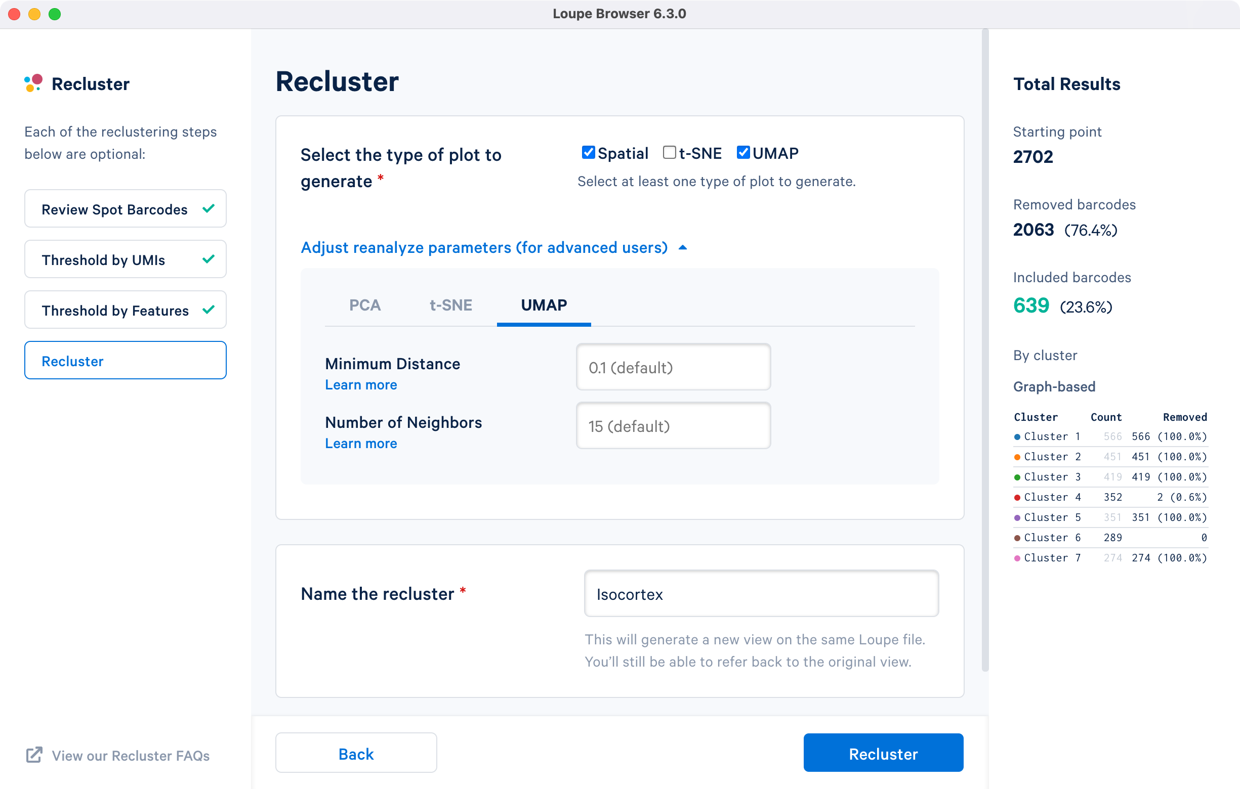
The final step in the workflow allows users to select the type of plot(s) to generate and to fine-tune the plotting parameters. By default, the spatial plot is selected for spatial datasets, with an additional choice of t-SNE and UMAP projections.
The drop down menu facilitates changing the default parameters for the dimensionality reduction used for clustering, or the parameters for generating the t-SNE and UMAP plots respectively. Click for additional information about parameter selection. Default parameter values are recommended. The last step is to name the reclustered dataset. The name will be used in the primary window as both the projection and clustering category. Adding the name unlocks the option. Note that duplication of Category names from the primary window are not allowed.
For the cluster-based selection, spatial plots and UMAP projections with default reanalyze parameters are selected and the dataset is named Isocortex.
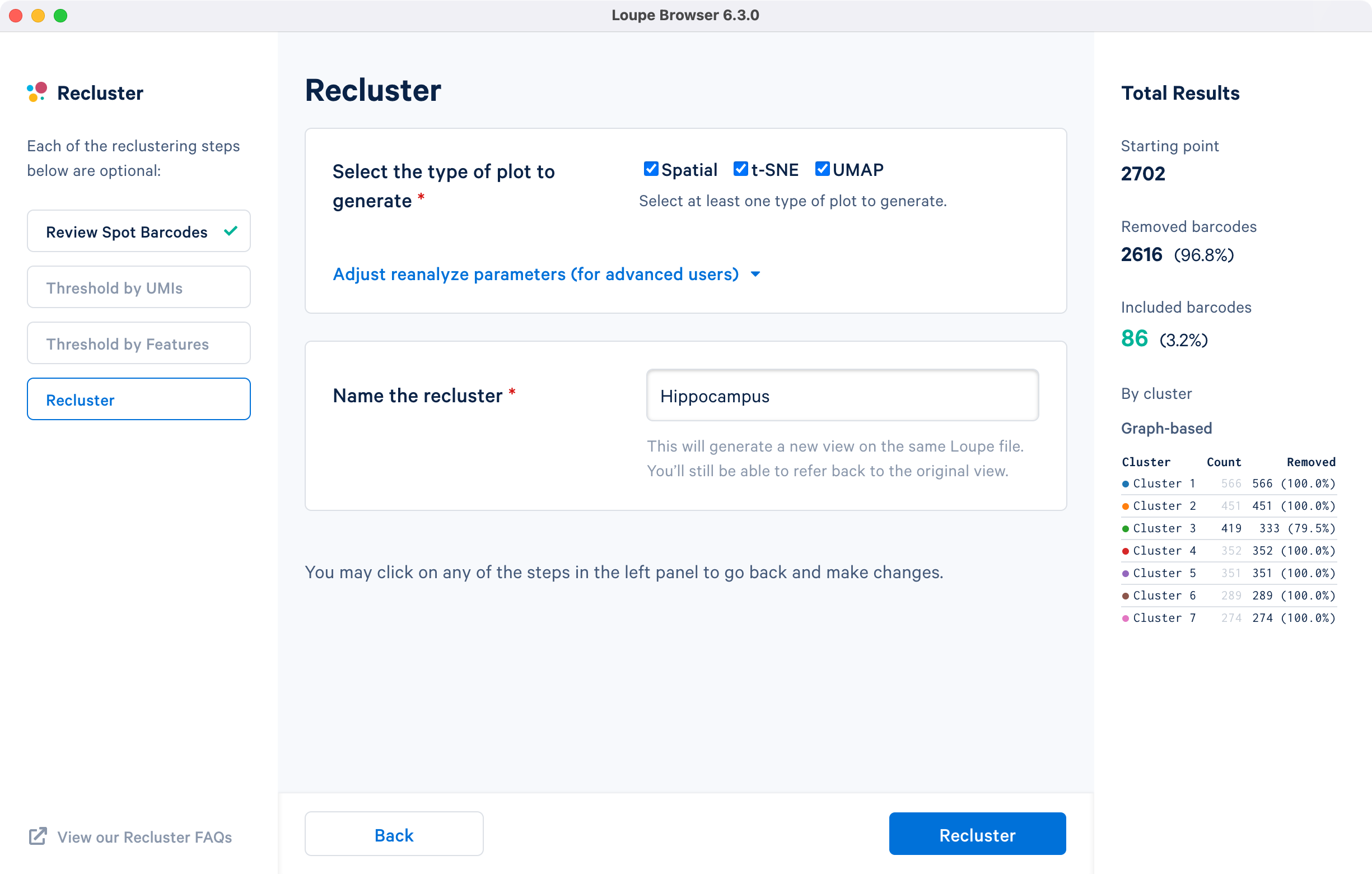
For the subregion-based selection achieved by uploading the CSV barcode file in Review Spot Barcodes step, all plot types are selected with default reanalyze parameters, and the dataset is named Hippocampus.
Click to initiate reclustering algorithms. In the background, Loupe will run virtually the same PCA, Louvain clustering, t-SNE, and UMAP algorithms as the Space Ranger pipeline.
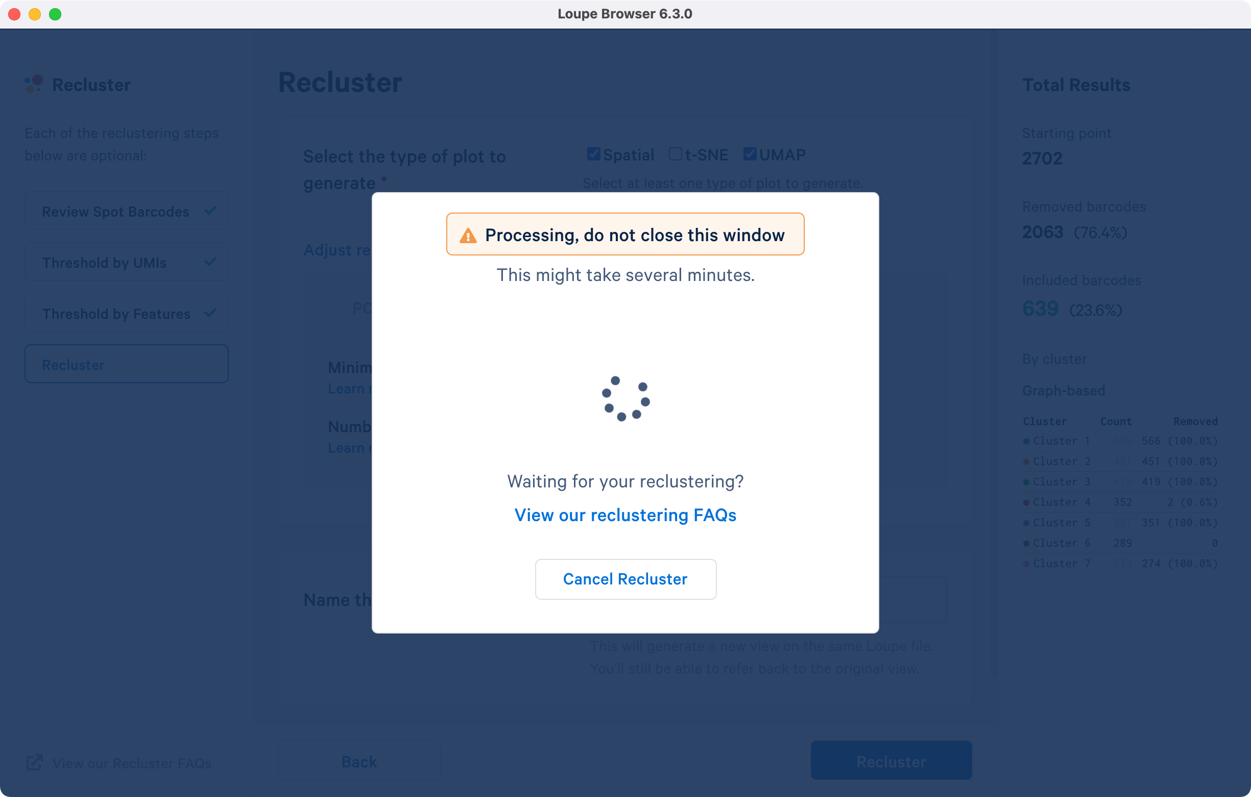
A successful completion of the reclustering workflow will result in updated text on the pop-up window.
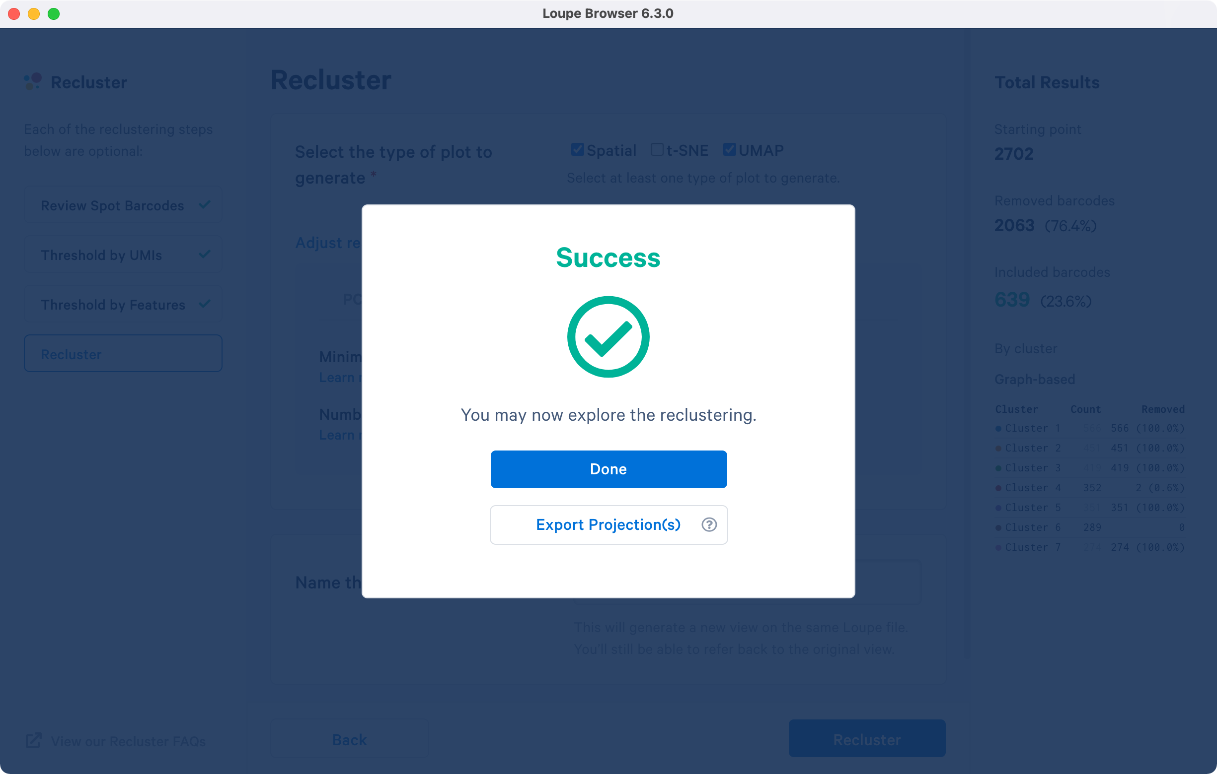
Selecting the will close the recluster window, and update the primary Loupe window to the new projection and category. Alternatively, export the projection coordinates of the spatial plot, t-SNE and/or UMAP projection(s) for the reclustered data by clicking . Selecting this option will follow the same steps as above in addition to downloading a .zip file to a local directory of your choice.
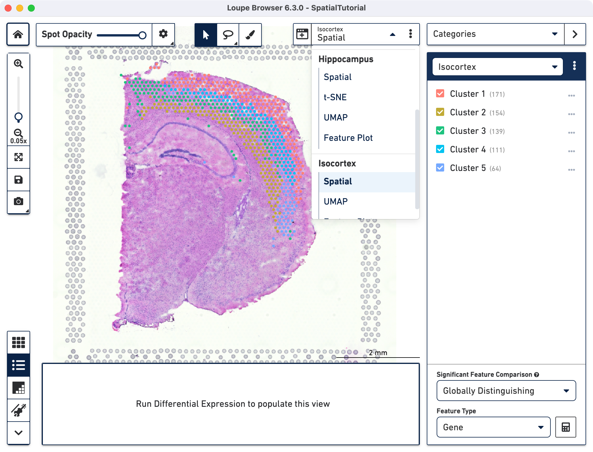
In the primary Loupe window, the reclustered plots appear under a separate category in the View Selector drop-down menu. To export the projection CSV file, click![]() in the View Selector panel for each plot type. Isocortex, the reclustered cluster-based dataset, is highlighted below. Note that more than one reclustered dataset can exist within the same Loupe file, with each listed under the unique name provided in the reclustering window.
in the View Selector panel for each plot type. Isocortex, the reclustered cluster-based dataset, is highlighted below. Note that more than one reclustered dataset can exist within the same Loupe file, with each listed under the unique name provided in the reclustering window.
All Loupe functions applicable to the full dataset are also applicable to the reclustered dataset, albeit restricted to only a subset of the spots from the original dataset. Users can open multiple linked windows, evaluate significant genes, and explore active features. Users can also visualize projections from reclustered datasets independently as well as projected onto the original dataset space.
As an example, consider the Isocortex, the reclustered dataset based on cluster selections in the original dataset. Note that the cluster colors were changed from default for clarity by clicking ![]() next to the cluster and selecting Edit Color. The original two clusters are now split into five distinct clusters. The clusters correspond closely to the following anatomical cortical layers:
next to the cluster and selecting Edit Color. The original two clusters are now split into five distinct clusters. The clusters correspond closely to the following anatomical cortical layers:
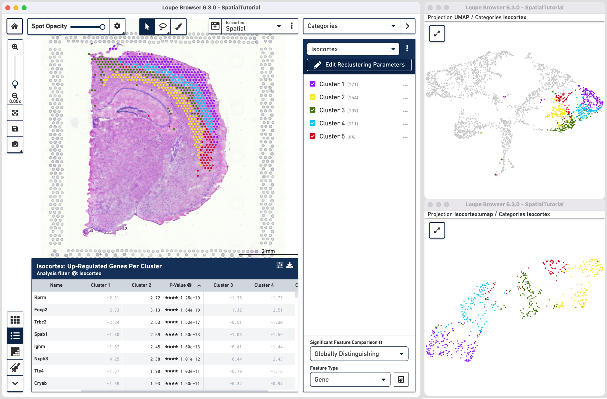
These results are further supported in the up-regulated gene feature table (e.g. Foxp2 is a layer 6 marker). The distinct molecular properties of the layers are also evident on the UMAP projections which show clear separation between the clusters.
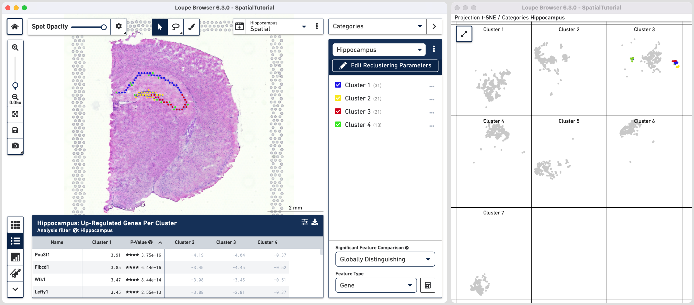
Hippocampus, the subregion-based reclustered dataset, is split into four distinct clusters. Cluster 1 corresponds to CA1, cluster 2 to dentate gyrus, and cluster 3 to CA2/CA3 subfields, respectively. Cluster 4 corresponds to signal from primarily non-neuronal cell types. This is further shown in the t-SNE projection on the original dataset which shows greater separation of cluster 4 relative to the other clusters. One of the top up-regulated genes in cluster 1 (Fibcd1), an established CA1 marker, was used to create Boolean filters in the Characterize Substructure tutorial.
Saving the .cloupe with the reclustered dataset follows the same rules as standard Loupe files and will save the reclustered projections and categories only, without any of the computed differential expression data. Finally, it is possible
to either tweak the reclustering or recall its parameters by clicking on which is located below any reclustered category.