Space Ranger2.0, printed on 11/17/2024
There may be some instances where loading Visium data into R would be helpful. These include viewing multiple genes at once for a sample or samples or viewing features for multiple samples at once including genes, UMIs, or clusters.
The following example shows how to plot this information to make figures of the following combinations:
| The following R code is designed to provide a baseline for how to do these exploratory analyses. These code-snippets are provided for instructional purposes only. 10x Genomics does not support or guarantee the code. |
First we load our libraries including Seurat, which provides easy functionality for reading the sparse matrix in h5 format:
library(ggplot2)
library(Matrix)
library(rjson)
library(cowplot)
library(RColorBrewer)
library(grid)
library(readbitmap)
library(Seurat)
library(dplyr)
library(hdf5r)
library(data.table)
The geom_spatial function is defined to make plotting your tissue image in ggplot a simple task.
geom_spatial <-  function(mapping = NULL,
                         data = NULL,
                         stat = "identity",
                         position = "identity",
                         na.rm = FALSE,
                         show.legend = NA,
                         inherit.aes = FALSE,
                         ...) {

  GeomCustom <- ggproto(
    "GeomCustom",
    Geom,
    setup_data = function(self, data, params) {
      data <- ggproto_parent(Geom, self)$setup_data(data, params)
      data
    },

    draw_group = function(data, panel_scales, coord) {
      vp <- grid::viewport(x=data$x, y=data$y)
      g <- grid::editGrob(data$grob[[1]], vp=vp)
      ggplot2:::ggname("geom_spatial", g)
    },

    required_aes = c("grob","x","y")

  )

  layer(
    geom = GeomCustom,
    mapping = mapping,
    data = data,
    stat = stat,
    position = position,
    show.legend = show.legend,
    inherit.aes = inherit.aes,
    params = list(na.rm = na.rm, ...)
  )
}
sample_names <- c("Sample1", "Sample2")
sample_names
Paths should be in the same order as the corresponding sample names.
image_paths <- c("/path/to/Sample1-spatial/tissue_lowres_image.png",
                 "/path/to/Sample2-spatial/tissue_lowres_image.png")

scalefactor_paths <- c("/path/to/Sample1-spatial/scalefactors_json.json",
                       "/path/to/Sample2-spatial/scalefactors_json.json")

tissue_paths <- c("/path/to/Sample1-spatial/tissue_positions_list.csv",
                  "/path/to/Sample2-spatial/tissue_positions_list.csv")

cluster_paths <- c("/path/to/Sample1/outs/analysis_csv/clustering/graphclust/clusters.csv",
                   "/path/to/Sample2/outs/analysis_csv/clustering/graphclust/clusters.csv")

matrix_paths <- c("/path/to/Sample1/outs/filtered_feature_bc_matrix.h5",
                  "/path/to/Sample2/outs/filtered_feature_bc_matrix.h5")
We also need to determine the image height and width for proper plotting in the end.
images_cl <- list()

for (i in 1:length(sample_names)) {
  images_cl[[i]] <- read.bitmap(image_paths[i])
}

height <- list()

for (i in 1:length(sample_names)) {
 height[[i]] <-  data.frame(height = nrow(images_cl[[i]]))
}

height <- bind_rows(height)

width <- list()

for (i in 1:length(sample_names)) {
 width[[i]] <- data.frame(width = ncol(images_cl[[i]]))
}

width <- bind_rows(width)
This step provides compatibility with ggplot2.
grobs <- list()
for (i in 1:length(sample_names)) {
  grobs[[i]] <- rasterGrob(images_cl[[i]], width=unit(1,"npc"), height=unit(1,"npc"))
}

images_tibble <- tibble(sample=factor(sample_names), grob=grobs)
images_tibble$height <- height$height
images_tibble$width <- width$width
scales <- list()

for (i in 1:length(sample_names)) {
  scales[[i]] <- rjson::fromJSON(file = scalefactor_paths[i])
}
clusters <- list()
for (i in 1:length(sample_names)) {
  clusters[[i]] <- read.csv(cluster_paths[i])
}
At this point, we also need to adjust the spot positions by the scale factor for the image we are using. In this case, we are using the lowres image, which has be resized by Space Ranger to be 600 pixels (largest dimension), but also keeps the proper aspec ratio.
For example, if your image is 12000 x 11000, the image is resized to 600 x 550. If your image is 11000 x 12000, the image is resized to 550 x 600.
bcs <- list()

for (i in 1:length(sample_names)) {
   bcs[[i]] <- read.csv(tissue_paths[i],col.names=c("barcode","tissue","row","col","imagerow","imagecol"), header = FALSE)
   bcs[[i]]$imagerow <- bcs[[i]]$imagerow * scales[[i]]$tissue_lowres_scalef    # scale tissue coordinates for lowres image
   bcs[[i]]$imagecol <- bcs[[i]]$imagecol * scales[[i]]$tissue_lowres_scalef
   bcs[[i]]$tissue <- as.factor(bcs[[i]]$tissue)
   bcs[[i]] <- merge(bcs[[i]], clusters[[i]], by.x = "barcode", by.y = "Barcode", all = TRUE)
   bcs[[i]]$height <- height$height[i]
   bcs[[i]]$width <- width$width[i]
}

names(bcs) <- sample_names
For the most simplistic approach, we are reading our filtered_feature_bc_matrix.h5 using the Seurat package. However, if you don't have access to the package, you can read in the files from the filtered_feature_be_matrix directory and reconstruct the data.frame with the barcodes as the row names, and the genes as the column names. See the code example below.
matrix <- list()

for (i in 1:length(sample_names)) {
 matrix[[i]] <- as.data.frame(t(Read10X_h5(matrix_paths[i])))
}
OPTIONAL: If you'd rather read from filtered_feature_bc_matrix directory instead of using Seurat. You can modify as above to write a loop to read these in.
matrix_dir = "/path/to/Sample1/outs/filtered_feature_bc_matrix/"
barcode.path <- paste0(matrix_dir, "barcodes.tsv.gz")
features.path <- paste0(matrix_dir, "features.tsv.gz")
matrix.path <- paste0(matrix_dir, "matrix.mtx.gz")
matrix <- t(readMM(file = matrix.path))
feature.names = read.delim(features.path,
                           header = FALSE,
                           stringsAsFactors = FALSE)
barcode.names = read.delim(barcode.path,
                           header = FALSE,
                           stringsAsFactors = FALSE)
rownames(matrix) = barcode.names$V1
colnames(matrix) = feature.names$V2
OPTIONAL: You can also parallelize this step using the doSNOW library if you are analyzing lots of samples.
library(doSNOW)

cl <- makeCluster(4)
registerDoSNOW(cl)

i = 1
matrix<- foreach(i=1:length(sample_names), .packages = c("Matrix", "Seurat")) %dopar% {
 as.data.frame(t(Read10X_h5(matrix_paths[i])))
}

stopCluster(cl)
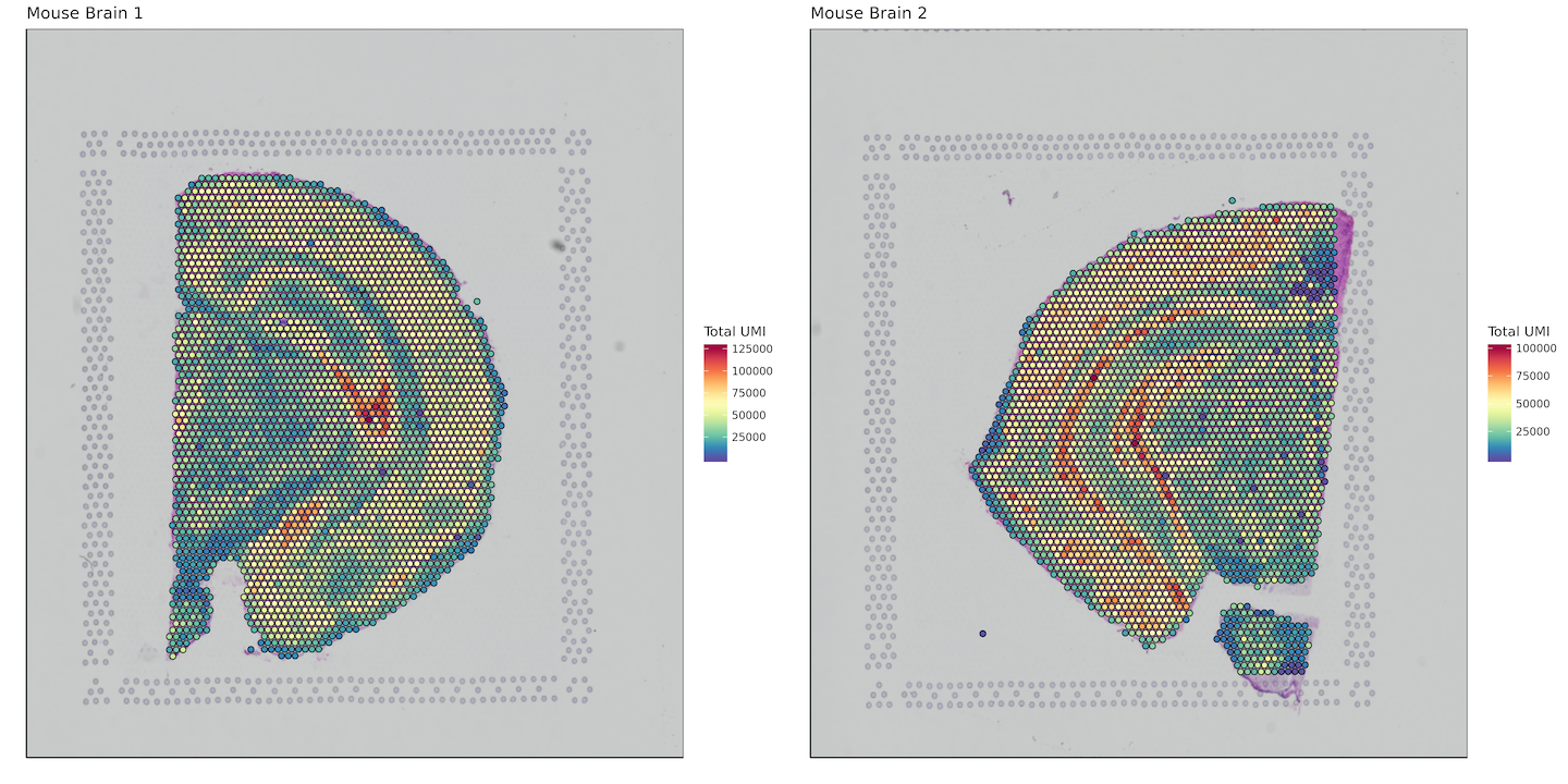
Total UMI per spot
umi_sum <- list()

for (i in 1:length(sample_names)) {
  umi_sum[[i]] <- data.frame(barcode =  row.names(matrix[[i]]),
                             sum_umi = Matrix::rowSums(matrix[[i]]))

}
names(umi_sum) <- sample_names

umi_sum <- bind_rows(umi_sum, .id = "sample")
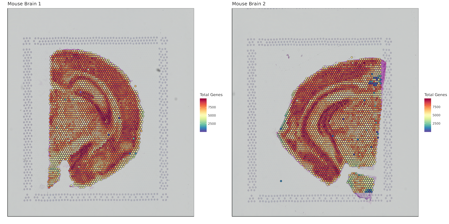
Total Genes per Spot
gene_sum <- list()

for (i in 1:length(sample_names)) {
  gene_sum[[i]] <- data.frame(barcode =  row.names(matrix[[i]]),
                             sum_gene = Matrix::rowSums(matrix[[i]] != 0))

}
names(gene_sum) <- sample_names

gene_sum <- bind_rows(gene_sum, .id = "sample")
In this final data.frame, we have information about your spot barcodes, spot tissue category (in/out), scaled spot row and column position, image size, and summary data.
bcs_merge <- bind_rows(bcs, .id = "sample")
bcs_merge <- merge(bcs_merge,umi_sum, by = c("barcode", "sample"))
bcs_merge <- merge(bcs_merge,gene_sum, by = c("barcode", "sample"))
We find that the most convenient way to plot lots of figures together is to make a list of them and utilize the cowplot package to do the arrangement.
Here, we'll take bcs_merge and filter for each individual sample in sample_names
We'll also use the image dimensions specific to each sample to make sure our plots have the correct x and y limits, as seen below.
xlim(0,max(bcs_merge %>%
          filter(sample ==sample_names[i]) %>%
          select(width)))
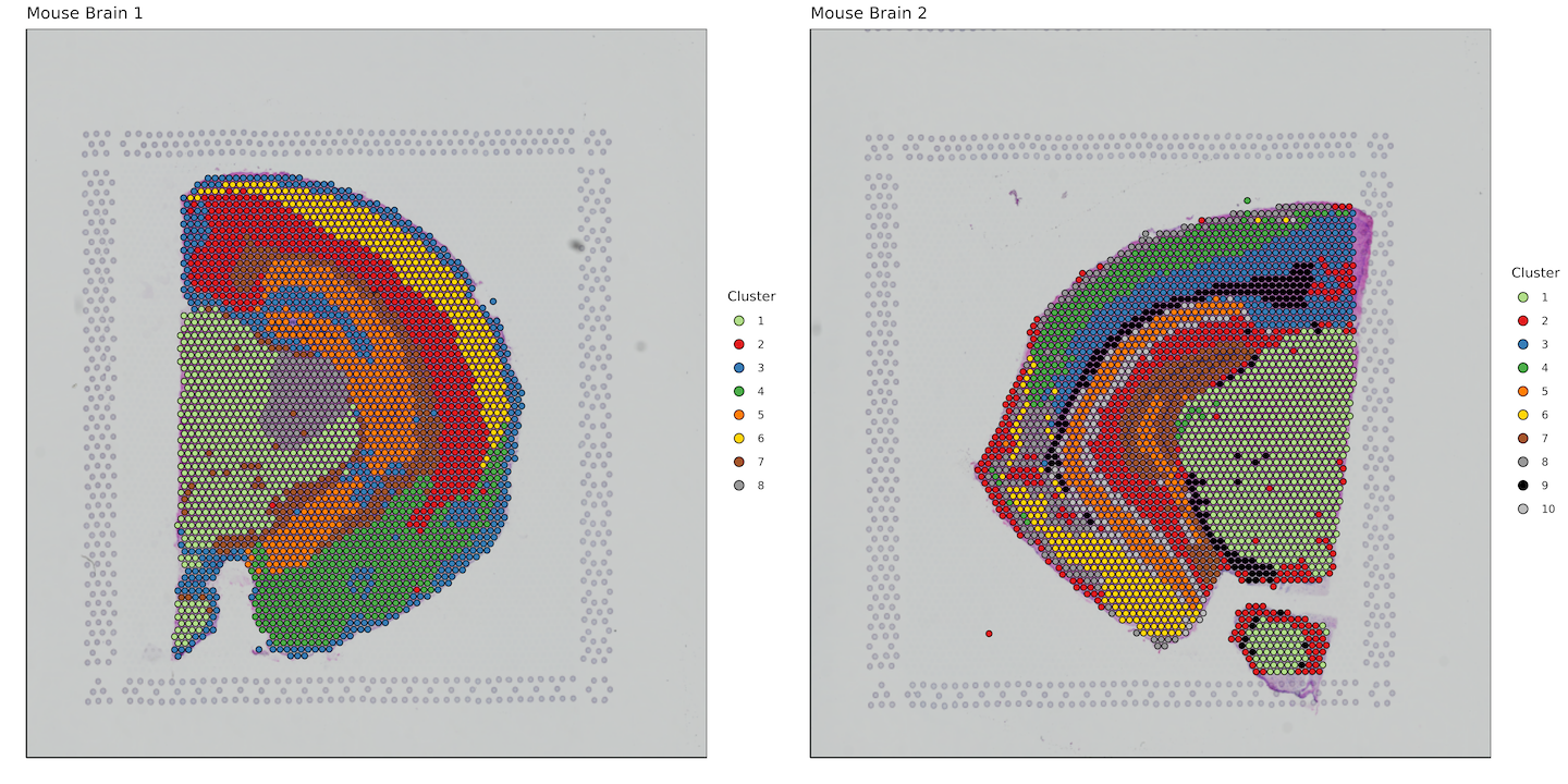
Note: Spots are not to scale
Define our color palette for plotting
myPalette <- colorRampPalette(rev(brewer.pal(11, "Spectral")))
plots <- list()

for (i in 1:length(sample_names)) {

plots[[i]] <- bcs_merge %>%
  filter(sample ==sample_names[i]) %>%
      ggplot(aes(x=imagecol,y=imagerow,fill=sum_umi)) +
                geom_spatial(data=images_tibble[i,], aes(grob=grob), x=0.5, y=0.5)+
                geom_point(shape = 21, colour = "black", size = 1.75, stroke = 0.5)+
                coord_cartesian(expand=FALSE)+
                scale_fill_gradientn(colours = myPalette(100))+
                xlim(0,max(bcs_merge %>%
                            filter(sample ==sample_names[i]) %>%
                            select(width)))+
                ylim(max(bcs_merge %>%
                            filter(sample ==sample_names[i]) %>%
                            select(height)),0)+
                xlab("") +
                ylab("") +
                ggtitle(sample_names[i])+
                labs(fill = "Total UMI")+
                theme_set(theme_bw(base_size = 10))+
                theme(panel.grid.major = element_blank(),
                        panel.grid.minor = element_blank(),
                        panel.background = element_blank(),
                        axis.line = element_line(colour = "black"),
                        axis.text = element_blank(),
                        axis.ticks = element_blank())
}

plot_grid(plotlist = plots)
plots <- list()

for (i in 1:length(sample_names)) {

plots[[i]] <- bcs_merge %>%
  filter(sample ==sample_names[i]) %>%
      ggplot(aes(x=imagecol,y=imagerow,fill=sum_gene)) +
                geom_spatial(data=images_tibble[i,], aes(grob=grob), x=0.5, y=0.5)+
                geom_point(shape = 21, colour = "black", size = 1.75, stroke = 0.5)+
                coord_cartesian(expand=FALSE)+
                scale_fill_gradientn(colours = myPalette(100))+
                xlim(0,max(bcs_merge %>%
                            filter(sample ==sample_names[i]) %>%
                            select(width)))+
                ylim(max(bcs_merge %>%
                            filter(sample ==sample_names[i]) %>%
                            select(height)),0)+
                xlab("") +
                ylab("") +
                ggtitle(sample_names[i])+
                labs(fill = "Total Genes")+
                theme_set(theme_bw(base_size = 10))+
                theme(panel.grid.major = element_blank(),
                        panel.grid.minor = element_blank(),
                        panel.background = element_blank(),
                        axis.line = element_line(colour = "black"),
                        axis.text = element_blank(),
                        axis.ticks = element_blank())
}

plot_grid(plotlist = plots)
plots <- list()

for (i in 1:length(sample_names)) {

plots[[i]] <- bcs_merge %>%
  filter(sample ==sample_names[i]) %>%
  filter(tissue == "1") %>%
      ggplot(aes(x=imagecol,y=imagerow,fill=factor(Cluster))) +
                geom_spatial(data=images_tibble[i,], aes(grob=grob), x=0.5, y=0.5)+
                geom_point(shape = 21, colour = "black", size = 1.75, stroke = 0.5)+
                coord_cartesian(expand=FALSE)+
                scale_fill_manual(values = c("#b2df8a","#e41a1c","#377eb8","#4daf4a","#ff7f00","gold", "#a65628", "#999999", "black", "grey", "white", "purple"))+
                xlim(0,max(bcs_merge %>%
                            filter(sample ==sample_names[i]) %>%
                            select(width)))+
                ylim(max(bcs_merge %>%
                            filter(sample ==sample_names[i]) %>%
                            select(height)),0)+
                xlab("") +
                ylab("") +
                ggtitle(sample_names[i])+
                labs(fill = "Cluster")+
                guides(fill = guide_legend(override.aes = list(size=3)))+
                theme_set(theme_bw(base_size = 10))+
                theme(panel.grid.major = element_blank(),
                        panel.grid.minor = element_blank(),
                        panel.background = element_blank(),
                        axis.line = element_line(colour = "black"),
                        axis.text = element_blank(),
                        axis.ticks = element_blank())
}

plot_grid(plotlist = plots)
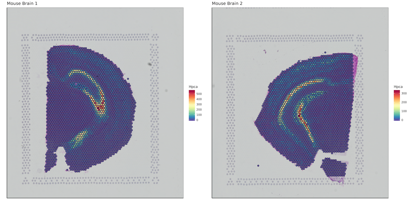
Here we want to plot a gene of interest, so we'll bind the bcs_merge data.frame with a subset of our matrix that contains our gene of interest. In this case, it will be the hippocampus specific gene Hpca. Keep in mind this is an example for mouse, for humans the gene symbol would be HPCA.
Converting to data.table allows for extremely fast subsetting as compared to using functions like dplyr::select().
plots <- list()

for (i in 1:length(sample_names)) {

plots[[i]] <- bcs_merge %>%
                  filter(sample ==sample_names[i]) %>%
                  bind_cols(as.data.table(matrix[i])[, "Hpca", with=FALSE]) %>%
  ggplot(aes(x=imagecol,y=imagerow,fill=Hpca)) +
                geom_spatial(data=images_tibble[i,], aes(grob=grob), x=0.5, y=0.5)+
                geom_point(shape = 21, colour = "black", size = 1.75, stroke = 0.5)+
                coord_cartesian(expand=FALSE)+
                scale_fill_gradientn(colours = myPalette(100))+
                xlim(0,max(bcs_merge %>%
                            filter(sample ==sample_names[i]) %>%
                            select(width)))+
                ylim(max(bcs_merge %>%
                            filter(sample ==sample_names[i]) %>%
                            select(height)),0)+
                xlab("") +
                ylab("") +
                ggtitle(sample_names[i])+
                theme_set(theme_bw(base_size = 10))+
                theme(panel.grid.major = element_blank(),
                        panel.grid.minor = element_blank(),
                        panel.background = element_blank(),
                        axis.line = element_line(colour = "black"),
                        axis.text = element_blank(),
                        axis.ticks = element_blank())
}

plot_grid(plotlist = plots)