Space Ranger4.0, printed on 03/29/2025
This tutorial reviews the major analysis capabilities Loupe Browser provides for analyzing data from the Visium Spatial Gene Expression solution. This example uses a mouse brain dataset that comes preloaded with Loupe Browser.
To use Loupe Browser, follow the directions on the Installation page to download and install the software on either macOS or Windows.
If you are new to Loupe Browser, learn more about the capabilities in the Navigation Tutorial.
Once you have installed Loupe Browser and are familiar with the basic navigation capabilities, you can start the Spatial Gene Expression tutorial to learn how to analyze data. Open Loupe Browser by double clicking on the application icon. Then click on the SpatialTutorial.cloupe file from the list of Recent Files.
Once you do that, you see a screen with the mouse brain image and the spots overlayed on top of the image. The spots are color-coded by the cluster that the spot was assigned to.
The Spatial Gene Expression dataset that is pre-bundled with Loupe Browser is a mouse brain sample from an E18 mouse.
There are a number of other Spatial Gene Expression datasets publicly available for download. These datasets include the .cloupe file that you can use to visualize the results. Visit the Spatial Gene Expression datasets page
This analysis tutorial shows you how to perform the following analyses using the functionality provided in Loupe Browser.
Goal: Evaluate the expression profiles of known gene markers of interest in the context of tissue morphology.
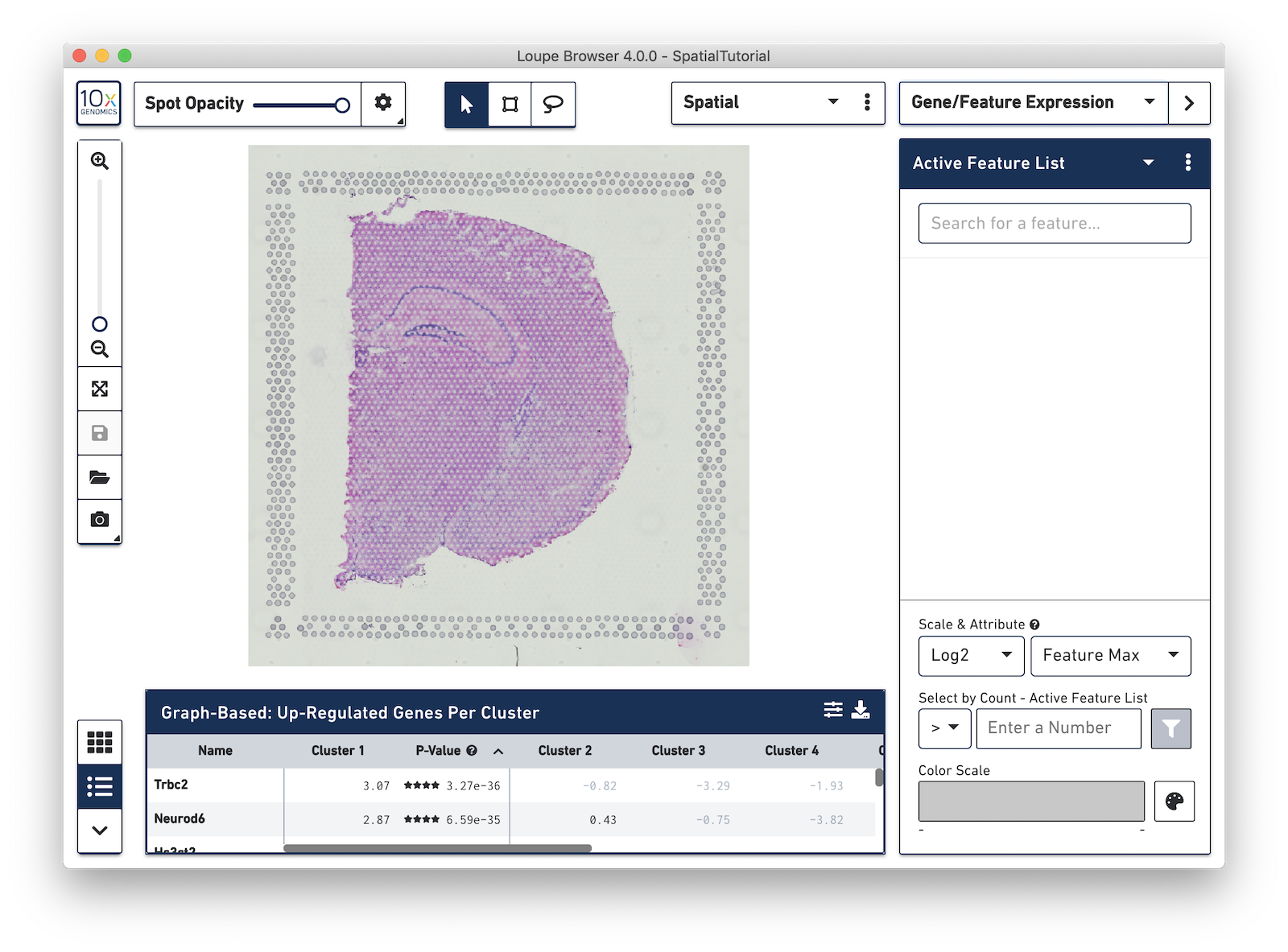
To effectively evaluate gene expression data in the context of the tissue image, it is helpful to understand the morphology and other information that can be uncovered from the tissue image. To do this, take the Spot Opacity slider, located in the top left hand corner, all the way to the left in order to remove the spots from the image.
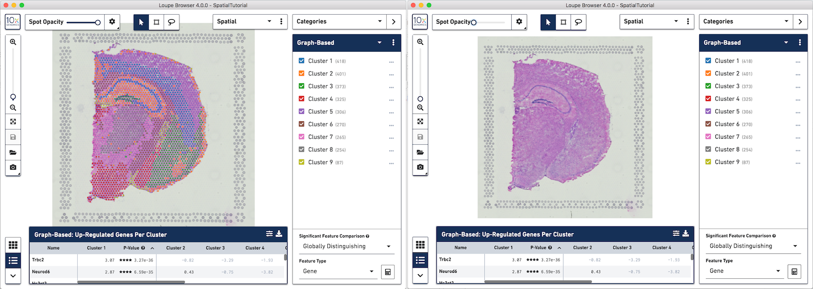
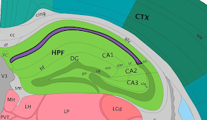
From there, you can use the zoom and mouse dragging functionality to navigate the image,evaluate the morphology, and identify landmarks of interest. For example, in this image, the curvature of the hippocampus is seen in the middle in blue.
Then type Rbfox3 into the text box. The auto-complete functionality helps to find genes of interest faster. Press Tab or Enter, to add the gene to the Active Feature List. The tissue image is then updated to color-code spots based on the level of Rbfox3 within that spot. High expression of the gene is indicated by a darker spot. In this example, Rbfox3 is expressed across the tissue, since it is a general neuronal gene marker. There is also a higher level of expression in the hippocampus and other parts of the cortex, as well as the thalamus and hypothalamus.
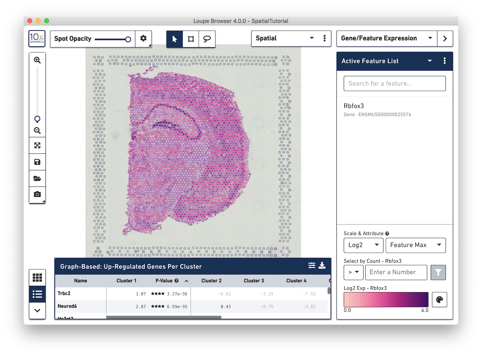
Note that some spots appear out of the range of the color scale, in this case, light gray. These are spots that show no expression of the gene. The color pallete in the bottom-right corner of the browser can be used to adjust the color-scale to meet your needs.
In the next example, search for the myelin basic protein (Mbp) gene that codes for one of the proteins in myelin, and add it to the Active Feature List. This is a marker for another cell type, oligodendrocytes, which produce the myelin sheaths that surround the axons of the neurons. As multiple features are added to the list, the color signature in the view represents a combination of expression levels across all the genes in the list.
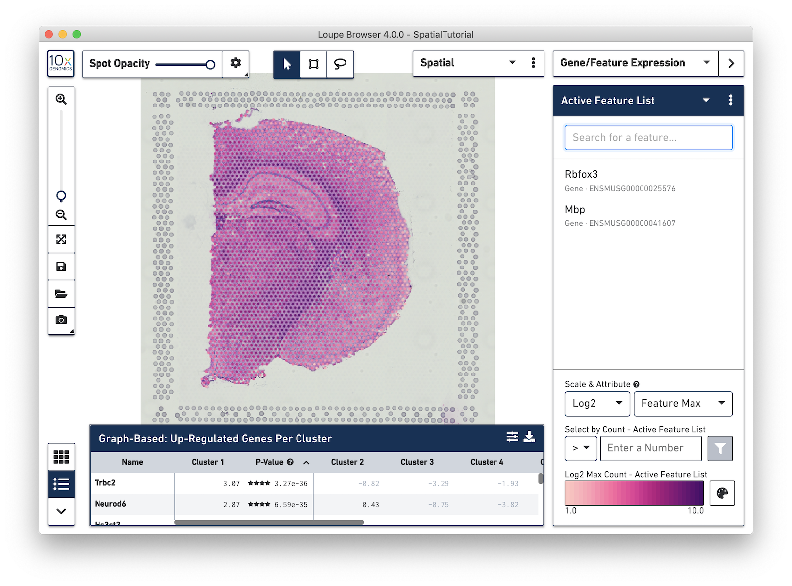
To see the expression pattern for only one of the genes in the Active Feature List, click on the gene name to select it. Click the gene name again to deselect it and revert back to visualizing the combination of expression levels. Hovering over a gene name reveals two icons, an information icon and a trash icon. Click the information icon to load the Ensembl reference page for that gene in a web browser. Click the trash icon to remove that gene from the current list.
![]()
By doing this, you can map known gene markers to spots, overlay that information on top of the tissue image, and use that to verify that the expected gene patterns are present in their respective brain tissue types.
Goal: Evaluating image data and clustering in the spatial view.
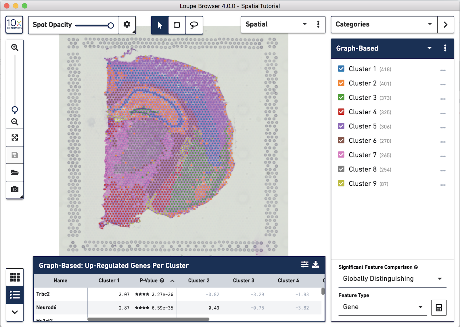
Spots that appear under the tissue are assigned to clusters by Space Ranger and are determined using only gene expression information, and without any spatial information from the image. Since each spot underneath the tissue is associated with a cluster, the clustering can be visualized in a spatial context. In this mouse brain sample, you can see how well the clustering follows the structure in the tissue.
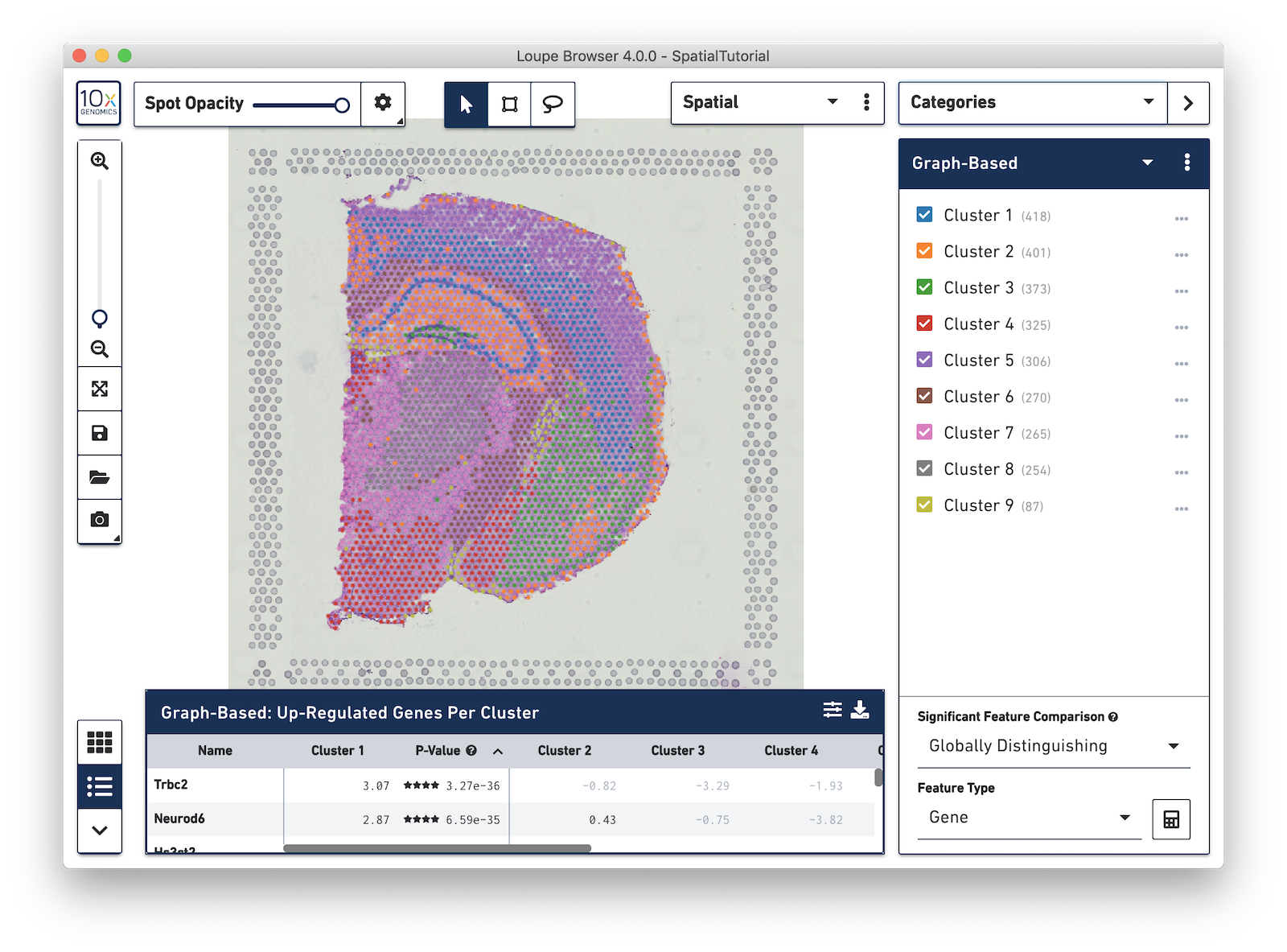
In this view, take a closer look at Cluster 1, in blue. It consists of a discontinuous selection of spots. When Spot Opacity is taken down to 0, the image shows that this cluster contains the hippocampus and part of the isocortex.
While Loupe Browser provides visualization of clusters determined by Space Ranger, it is possible to define your own clusters based on gene markers. In this example, the Import List functionality is used to do that. Click here to download list of genes that correspond to the CA1, CA2 and CA3 regions of the hippocampus. This file contains the following genes:
Note that the gene names must match with the ones included in the annotation
reference provided to spaceranger count. See the
Import Lists section of the Navigation tutorial to
learn more about how to construct your own lists.
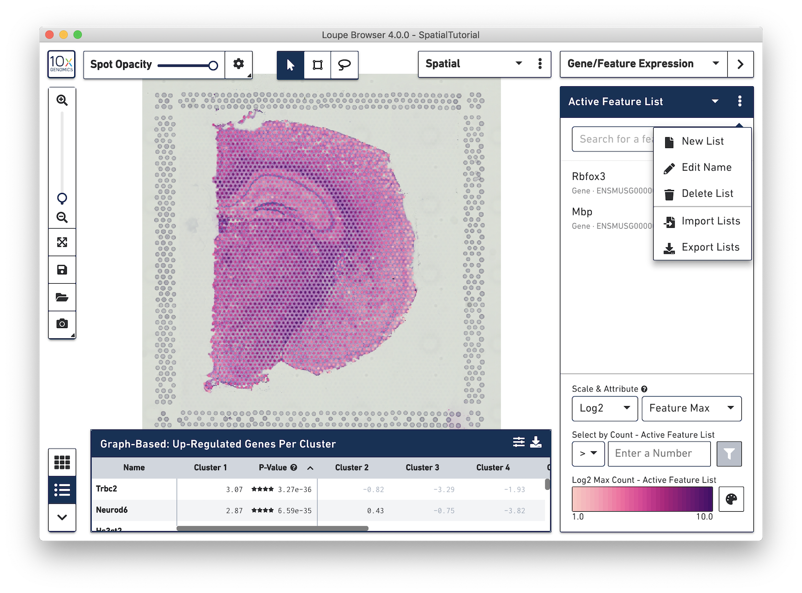
To import the csv file into Loupe Browser, you must be in the Gene/Feature Expression mode. From here, click on the three dots to the right of the Active Feature List and select Import Lists from the drop-down menu.
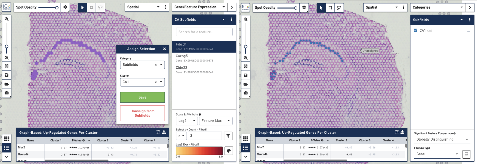
After it is imported, a new gene list called CA Subfields will be visible, with the three hippocampal gene markers in the list. For this section of the tutorial, we will be focusing on the CA1 subfield of the hippocampus. The gene Fibcd1 is a marker for this subfield; click on the Fibcd1 to see expression of that single gene. The spots that are most highly expressive of that gene show up as darker red in the graphic below. Fibcd1 is concentrated in the CA1 region of the hippocampus and the habenula.

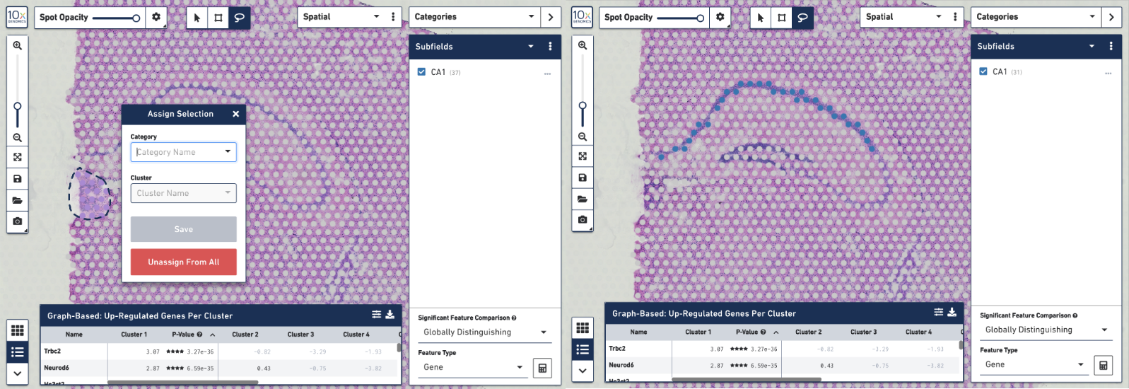
To create your own CA1 cluster, first filter the spots to select for only the ones that are highly expressive of the Fibcd1 gene. Based on the coloring of spots and the Log2 Max Count scale at the bottom of the Gene Expression panel, we will set a threshold of 3. Enter 3 into the Select By Count field above the Log2 Max Count scale and click on the filter button. This gives us the option to create a new cluster that contains only those spots. The spots which were selected by the filter are highlighted in purple in the background. You can create a new Category name called Subfields and a new Cluster name called CA1. Once this is saved, you are taken to Category mode. The Subfields category is displayed along with the new Cluster, CA1, that we just created.
We know that some of the spots assigned to the cluster are in fact not part of the CA1 region of the brain. In order to have a pure cluster, you can remove the spots that are associated with the habenula. To do this, use the lasso tool to select the spots in the habenula. Then, in the pop-up menu, click Unassign from All. Once this is done, only the spots that fall on the CA1 region of the hippocampus remain in the cluster.
Goal: To find subgroups within the clusters and perform differential gene expression.
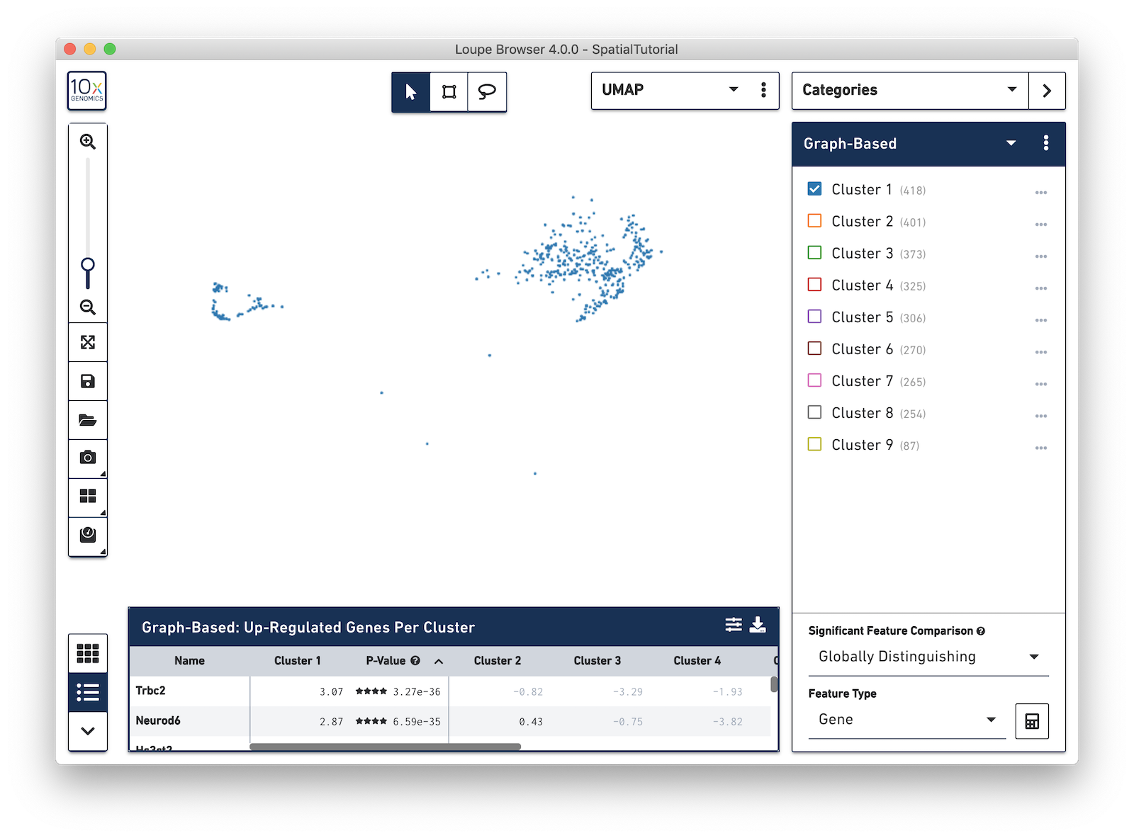
In addition to projecting the spots and their associated clusters onto the image, the clustering can also be viewed as a t-SNE or UMAP projection. In this example, look at the UMAP projection by using the View Selector and switching to UMAP. The default clustering results used in this view are from the Graph-based clustering method. The size of the spots can be adjusted to make them easier to see. See the Toolbox description in the Navigation tutorial.
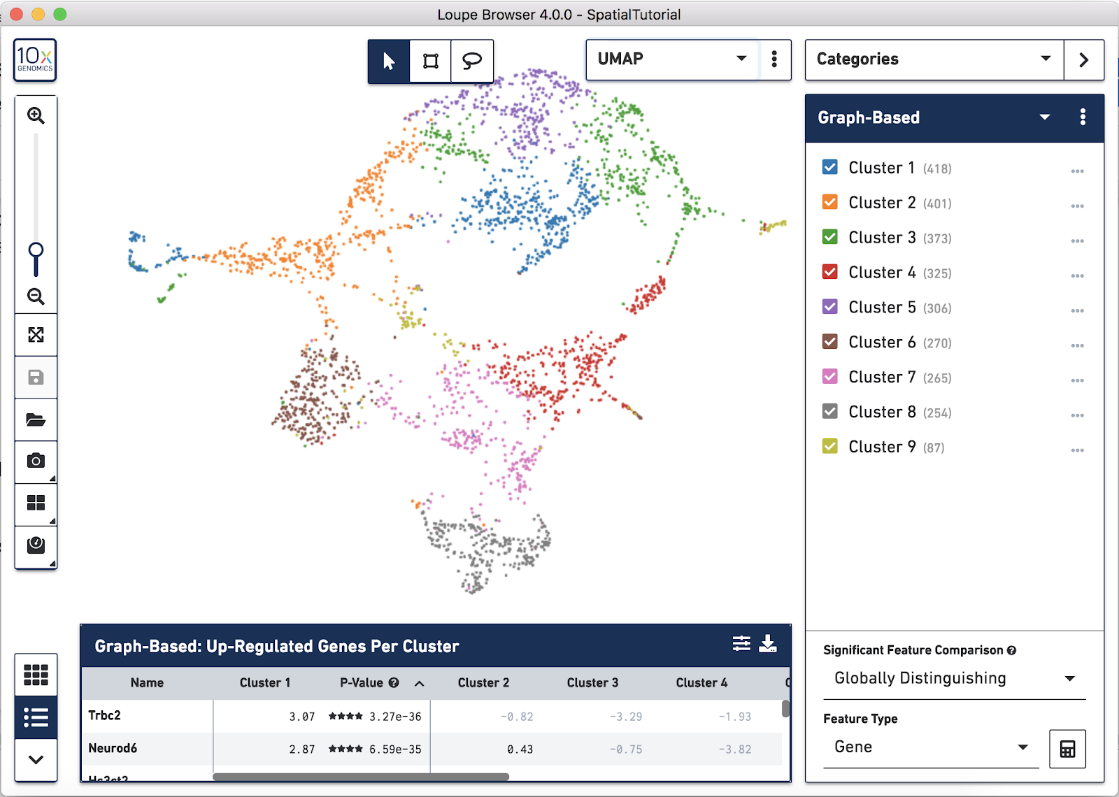
Now focus on Cluster 1 to see that there are two visually distinct sub-populations. To do this, uncheck all of the other clusters.
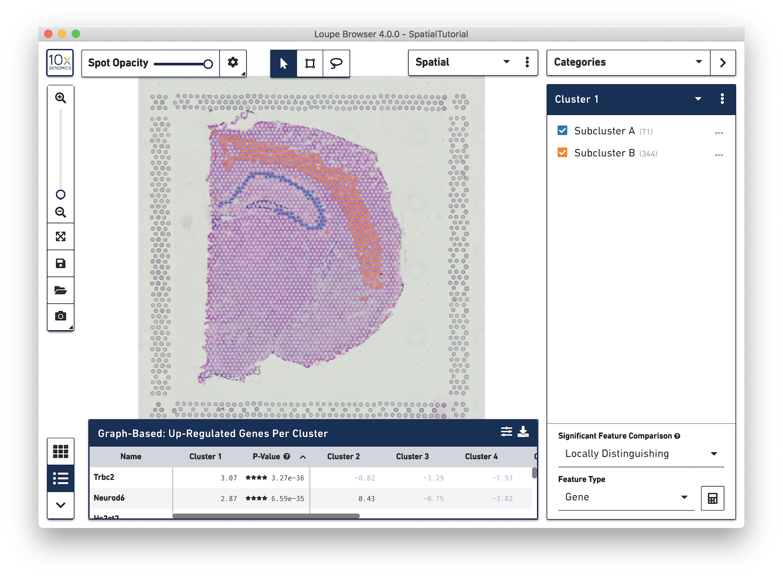
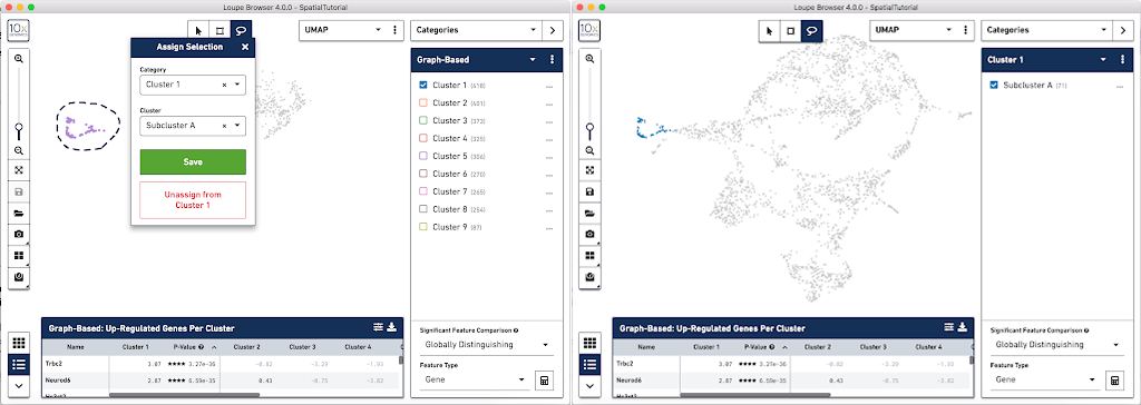
In order to explore these two sub-clusters more, create new groups, one for each sub-cluster. To do this, use the lasso tool to manually select one group of spots, create a new Category called Cluster 1 and a new Cluster name called Subcluster A.
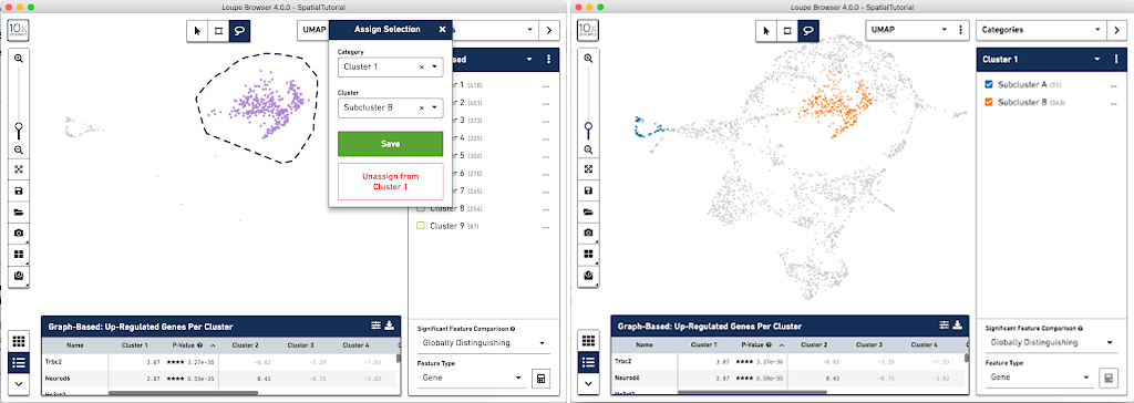
From this Cluster 1 view, go back to the Graph-Based view and do the same thing with the other subgroup of spots. First associate them with the same category, Cluster 1, but name the cluster Subcluster B.
From here, conduct differential gene expression analysis between the two Subclusters. To do this, choose the Locally Distinguishing option from the Significant Feature Comparison selector in the bottom right. See the Significant Feature Comparison explanation in the Navigation tutorial for more details.
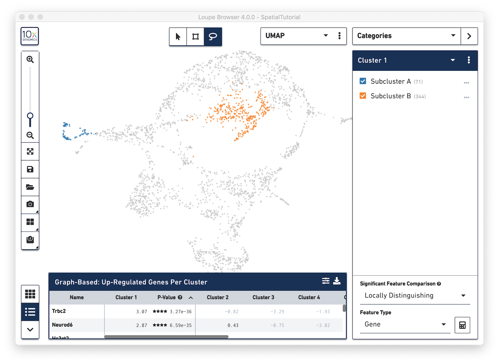
Look at the Data Panel on the bottom to see the top differentially expressed genes between these two Subclusters. Use the settings icon in the right-hand corner of the table to control the values displayed in the Data Panel.
Any custom categories and clusters that are manually defined can also be visualized in the Spatial View. Use the View Controller to switch from the UMAP view to the Spatial View. We are still looking at the custom category called Cluster 1 and the two sub-clusters manually defined. You can quickly see that these two sub-clusters align nicely to two distinct landmarks in the tissue. Subcluster A corresponds to the Hippocampus and Subcluster B corresponds to the isocortex.