Cell Ranger DNA1.1, printed on 04/02/2025
| Analysis software for the 10x Genomics single cell DNA product is no longer supported. Raw data processing pipelines and visualization tools are available for download and can be used for analyzing legacy data from 10x Genomics kits in accordance with our end user licensing agreement without support. |
Genomic heterogeneity is the hallmark of many complex diseases, including cancer, that are characterized by cellular subpopulations evolving distinct genotypes and phenotypes. The ability to accurately assess and investigate the clonal makeup of these diseases is limited when using traditional bulk methods such as whole-genome sequencing and microarrays. Single-cell DNA sequencing is a powerful method to resolve genomic heterogeneity by building deep profiles of individual cells that otherwise get masked.
This tutorial leverages the new and improved features of Cell Ranger DNA 1.1 and Loupe scDNA Browser 1.1 using two new datasets:
Email support@10xgenomics.com with any questions or concerns about this tutorial or the scCNV solution. Your success is important to us.
In this tutorial, you will learn how to:
You need access to a Linux machine to run the Cell Ranger DNA 1.1 pipeline. See system requirements. If you don’t have access to adequate computational resources, you can still complete the QC and visualization portions of this tutorial.
You also need access to a Windows or Mac machine to run Loupe scDNA Browser.
Download the following:
Follow the instructions here to install the pipeline, check your machine's specifications and do a test run. Email support@10xgenomics.com with any problems or questions.
Once Cell Ranger DNA is installed on your Linux machine, check the path by entering cellranger-dna on the command line. A message similar to the following is returned:
[user.name@server COLO829]$ cellranger-dna
cellranger-dna  (1.1.0)
Copyright (c) 2019 10x Genomics, Inc.  All rights reserved.
------------------------------------------------------------------------------

Usage:
cellranger-dna mkfastq
cellranger-dna cnv
cellranger-dna aggr
cellranger-dna reanalyze
cellranger-dna mkref
cellranger-dna bamslice
cellranger-dna testrun
cellranger-dna upload
cellranger-dna sitecheck
[user.name@server COLO829]$
Next, download the FASTQ files. These files represent data from 1,475 G1 sorted COLO829 cells obtained from the American Type Culture Collection (ATCC). There are 3.04 billion Novaseq reads from two flowcells with a read construct of 100 (R1), 8 (i7), 100 (R2). You can use the following command to download the tarball:
wget https://cf.10xgenomics.com/samples/cell-dna/1.0.0/colo829_G1_1k/colo829_G1_1k_fastqs.tar
Once the data is unpacked, run the pipeline on the fastq data with the following command:
cellranger-dna cnv --id=COLO829G1 \
--fastqs=/path/to/colo829_G1_1k_fastqs_demux/H35TCDSXX/ \
--reference=/path/to/refdata-GRCh38-1.0.0 \
--localmem=128 \
--localcores=16
Note: For the purpose of this tutorial, only data from one of the two flowcells is used.
Important: By default, Cell Ranger DNA runs in --jobmode=local and uses 90% of the available memory and all available cores. This can sometimes cause problems, especially on a shared server or cluster. In this example, we set --localmem=128 and --localcores=16 to request 128 GB of RAM and 16 cores. These are the minimum requirements of the Cell Ranger DNA pipeline, and can be scaled up as needed.
Important: When submitting a job to a cluster or cloud, especially a shared resource with a batch-queue system like LSF or SGE, you may need to request at least this many resources in your jobscript or command line. See How do I run and troubleshoot 10x pipelines on a HPC cluster?
The --id argument merely names the output directory and shows up in the web_summary.html file. Normally, we recommend that you make this as informative as necessary with standard characters.
Be sure to replace /path/to with the actual full path to your FASTQ files and reference.
Tip: Type pwd to get the full path to the current working directory.
Once the run is completed, navigate to the outs directory.
Open the web_summary.html file in a web browser, and start with the key metrics displayed on top.
Estimated Number of Cells: This can be compared to the estimated number of cells captured in the lab.
Median estimated CNV resolution (in Mb): This shows the smallest event that can be detected in a single cell. In this experiment the event resolution was 1.58 Mb. A CNV resolution of 2 Mb can be detected at a sequencing depth of 750k read pairs/cell in human samples.
Median ploidy: Each cell has an average ploidy. This is the median of those averages. For the underlying math, see the section on scale factor estimation on the CNV algorithms page.
Sequencing
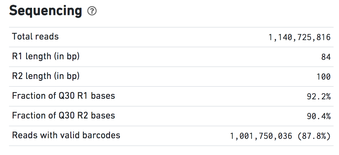
Make sure that the total number of reads matches with what is expected. In this dataset there are 1.14 billion NovaSeq paired end reads.
Note that the sequencing was 100 x 100 following standard sequencing requirements, but the first 16 bases, the 10x barcode that identifies the droplet, are trimmed from Read 1.
Cells and Mapping
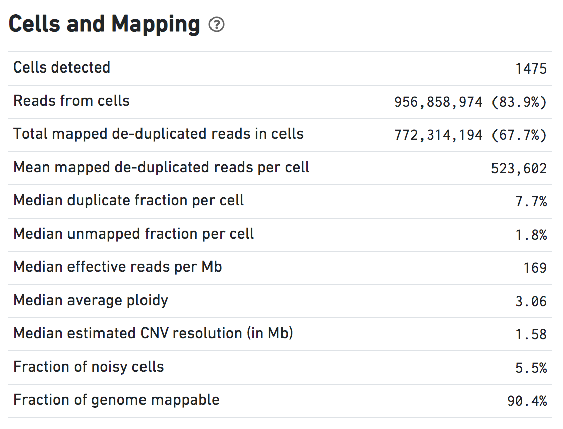
Click the question mark symbol for definitions of these metrics.
Total mapped de-duplicated reads in cells are non-duplicate, MAPQ > 30 reads used for CNV calling. Typical range: >60% of the Total Reads.
Median duplicate fraction per cell reflects reads lost due to PCR duplication and diffusion duplication during sequencing. Typical range: <15%.
Median unmapped fraction per cell reflects overall data quality. These are data from only the detected cells, not the background reads. Typical range: <1%.
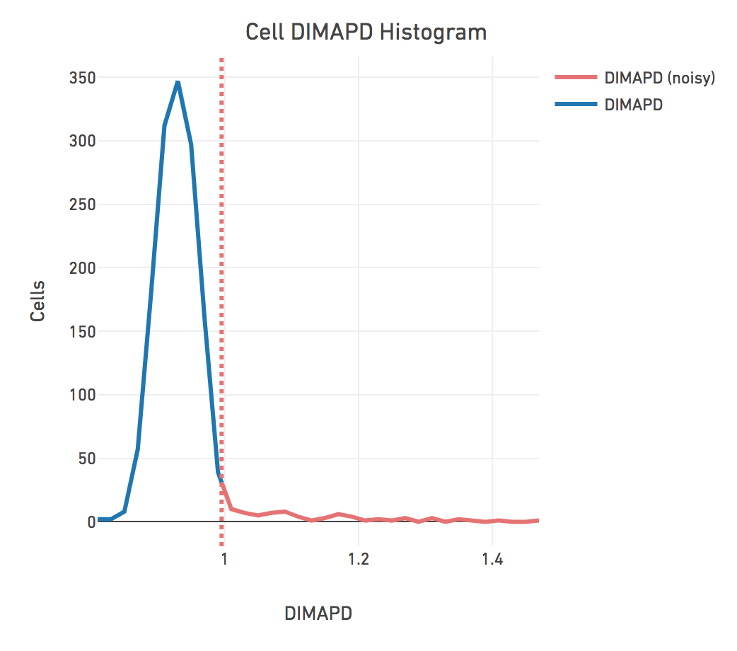
A cell is classified as noisy if the ploidy_confidence from CNV calling is low or if the DIMAPD value is an outlier compared to the rest of the sample population. See below.
Cell Plots
This is a histogram of barcodes ranked by mapped reads. A clean dataset should have a single steep cliff or drop off demonstrating the separation of signal (droplets containing cells) from noise (empty droplets), as seen below.
The green portion on the left is mapped reads in cells, that are retained for subsequent analyses.
Note that both axes are on a logarithmic scale. Most barcodes called as cells have >1M mapped reads, in contrast to barcodes called as empty droplets which have <10K mapped reads. A double peak or gradual decline may indicate technical issues like GEM coalescence or poor cell viability.
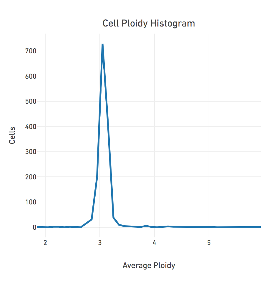
The Cell Ploidy Histogram shows the Average Ploidy distribution across the cells in the dataset. The example below shows that most cells have an estimated ploidy around 3.
DIMAPD
Depth-Independent Median Absolute deviation of Pairwise Differences (DIMAPD) measures the bin-to-bin deviation of read depth in a cell, perturbed by biological or technical variability. It is one of two methods to detect noisy cells. The other method is that the ploidy_confidence was low. Most of the cells should have a DIMAPD below the threshold for noisy cells marked by the dashed red line as seen here.
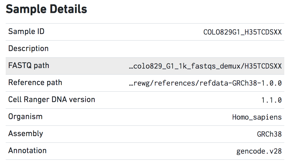
Sample Details
Sample Details are useful for keeping track of the parameters of different runs. The Sample ID, FASTQ path, and Reference path represent the --id, --fastqs, and --reference arguments, respectively.
Next, look at some of the other output files.
Look at some other potentially useful output files in the outs directory.
[user.name@server outs]$ ls
alarms_summary.txt  mappable_regions.bed         per_cell_summary_metrics.csv  summary.csv
cnv_data.h5         node_cnv_calls.bed           possorted_bam.bam             web_summary.html
dloupe.dloupe       node_unmerged_cnv_calls.bed  possorted_bam.bam.bai
The per_cell_summary_metrics.csv contains various metrics that provide per-cell information, and is easily visualized in Excel or another similar program.
The summary.csv file is a recapitulation of the metrics presented in the web_summary.html file. This file is mainly useful for keeping track of multiple experiments.
The node_cnv_calls.bed file is a six column tab-separated file that contains the CNV calls for each cell and group in the tree.
[user.name@server outs]$ head node_cnv_calls.bed
#cellranger-dna 1.1.0
#reference genome: /mnt/yard1/andrewg/references/refdata-GRCh38-1.0.0
#chrom  start   end     id      copy_number     event_confidence
chr1    820000  840000  2842    7       0
chr1    820000  840000  2906    3       48
chr1    820000  840000  2910    3       48
chr1    820000  840000  2918    3       47
chr1    820000  840000  2922    3       56
chr1    820000  860000  1558    7       0
chr1    820000  860000  2587    0       5
The mappable_regions.bed file is a three-column tab-separated file containing the mappable regions.
[user.name@server outs]$ head mappable_regions.bed
#cellranger-dna 1.1.0
#reference genome: /mnt/yard1/andrewg/references/refdata-GRCh38-1.0.0
#chrom  start   end
chr1    820000  1640000
chr1    1660000 1680000
chr1    1720000 2660000
chr1    2780000 12860000
chr1    13100000        13120000
chr1    13220000        13240000
chr1    13360000        16540000
The possorted_bam.bam file is in standard BAM format. The corresponding index file (.bai) is also provided. The BAM also includes 10x specific tags for the cellular barcode (both raw and error-corrected against the whitelist), a sample index, and base qualities for both. This file is also used as input for the cellranger-dna bamslice pipeline, which is covered below.
The BAM file is binary and not human readable, but can be read using a tool like samtools (bundled with Cell Ranger DNA) to view the BAM file.
[user.name@server outs]$ source /mnt/yard1/andrewg/cellranger-dna-1.1.0/sourceme.bash
[user.name@server outs]$ samtools view possorted_bam.bam | head
A00228:141:H35TCDSXX:2:1327:23339:30326 147 chr1    9993    0   9S91M   =   10027   -57 TCTCTATCCCTGTCCGGTAACCCTAACCCTAACCCTAACCCTAACCCTAACCCTAACCCTAACCCTAACCCTAACCCTAACCCTAACCCTAACCCTAACC    FF:F,,F,F,,,,,F,,,FFFFFFFFFFFFFFFFFFFFFFFFFFFFFFFFFFFFFFFFFFFFFFFFF:FFFFFFFFFFFFFFFFFFFFFFFFFFFFFFFF    NM:i:1  MD:Z:7A83   AS:i:86 XS:i:84 GP:i:10083  MP:i:10026  BC:Z:ACAAGGTA   QT:Z:FFFFFFFF   CR:Z:CTAGCCTTCTCCGGAA   CY:Z:FFFFFFFFFFFFFFFF   RG:Z:COLO829G1_H35TCDSXX:LibraryNotSpecified:1:H35TCDSXX:2  CB:Z:CTAGCCTTCTCCGGAG-1
The cnv_data.h5 file is in the HDF5 file format is designed to manage and store large datasets. It is structured similar to a dictionary, with a series of keys storing values. This file is necessary to run both cellranger-dna reanalyze and cellranger-dna aggr. It is a binary file, so it cannot be viewed without special tools.
Open the dloupe.dloupe file in the Loupe scDNA Browser and take time to orient yourself with the major features. We recommend completing the original MKN-45 tutorial that introduces these major features of the browser first.
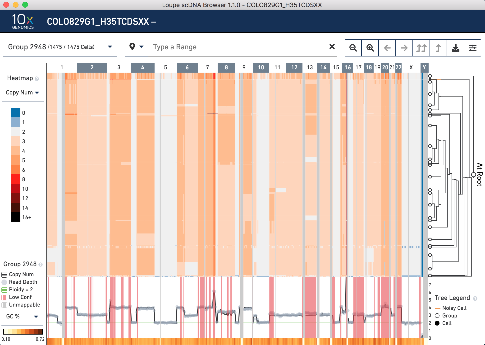
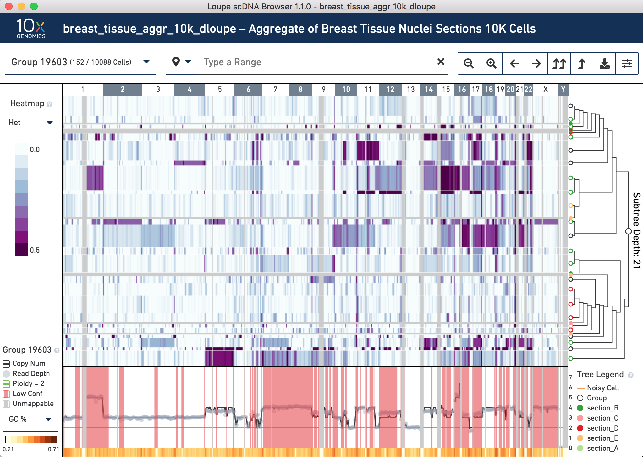
The center of the screen is the heatmap view. The chromosomes are arranged along the top of the heatmap. Click any one of them to zoom in. The colors in the heatmap correspond with the legend to the left, and are adjustable. Above the chromosomes, one can navigate by group,vertically (corresponding with the tree on the right) and horizontally, by genomic region. There are other navigation buttons as well. To the right of the heatmap is the hierarchical clustering tree. Click nodes (where two branches join) or leaves (tips of the tree) to navigate to groups or cells. The base of the tree is called the root. Not all cells can be displayed in the view simultaneously. There are options in the top view for how many nodes to display at a time. The tree legend indicates groups and noisy cells. To the bottom of the heatmap is the view of copy number, read depth, unmappable regions, and low confidence regions. There is also a smaller heatmap displaying either GC content or heterogeneity across the genome.
Velazquez-Villarreal et al. (2019) found large CNVs on chromosomes 1, 10 and 18 that were maintained in all but two groups. These two groups carried a loss of one copy of chromosome 8. Are these CNVs present in the .dloupe file? Yes. However, they are not directly viewable as shown in the paper. There are two reasons for this. First, at this stage, it is not obvious which cells in the .dloupe file correspond to which groups (subclones) in the paper. Second, there are cells in the dataset that are identified as noisy. This could be due to either technical noise, or a true biological rare clone with replicating cells.
To overcome these, the next section of the tutorial focuses on running cellranger-dna reanalyze to impose grouping constraints on clustering derived from the manuscript and to remove noisy cells as described above. This enables us to better examine these CNVs with the Loupe scDNA Browser.
Before running cellranger-dna reanalyze, consider groups A-D in Figure 3 adapted from Velazquez-Villarreal et al. (2019).
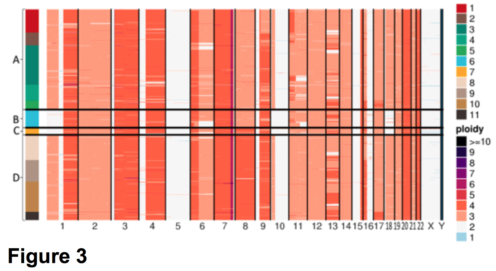
In the left pane in Figure 3, cells are stacked according to four distinct groups, A-D, that were identified through Discriminant Analysis of Principal Components (DAPC). DAPC is beyond the scope of this tutorial. Refer to the paper for additional details. A list of barcodes in each group is provided in Supplementary Table 3. We use these barcodes to constrain the analysis so that the four groups cluster together and can be compared to the new .dloupe file to Figure 3. To run cellranger-dna reanalyze, download the necessary CSV files here, unpack the tarball (tar -xfz COLO829reanalyzefiles.tgz), and look inside.
There are four CSV files for each group:
groupA.csv
groupB.csv
groupC.csv
groupD.csv
These are directly derived from Supplemental Table 3. Additionally, noisy cells were removed based on whether they were flagged as noisy in the per_cell_summary_metrics.csv file.
For example, the first five lines of groupA.csv are five cell barcodes as follows:
AAACCTGAGGCTACGA-1
AAACCTGGTCCTTGGG-1
AAACGGGAGCAGATCG-1
AAACGGGCAAAGTAAC-1
AAACGGGCAACCTCAA-1
The reanalyze_config.csv tells Cell Ranger DNA what the four groups are and where to find the CSV files listed above.
library_id,barcodes_csv
groupA,groupA.csv
groupB,groupB.csv
groupC,groupC.csv
groupD,groupD.csv
The constraint.tre file specifies the guide tree —-how the four groups are related to each other. Since the true phylogeny is not known in this case, it is assumed that B and C are sister to each other, in turn sister to group A, with group D as the outgroup.
(((groupB,groupC),groupA),groupD);
After uploading these CSV and newick files to the Linux server, run cellranger-dna reanalyze as shown below. Be sure to replace /path/to with the actual full path to each file. Note that the input data to be reanalyzed is the cnv_data.h5 file as discussed above.
cellranger-dna reanalyze --id=COLO829_reanalyzed \
--reference=/path/to/refdata-GRCh38-1.0.0 \
--tree=/path/to/constraint.tre \
--cnv-data=/path/to/cnv_data.h5 \
--csv=/path/to/reanalyze_config.csv \
--localmem=128 \
--localcores=16
Once the run is completed, open the new .dloupe file which is located in the outs directory. What are some key differences?
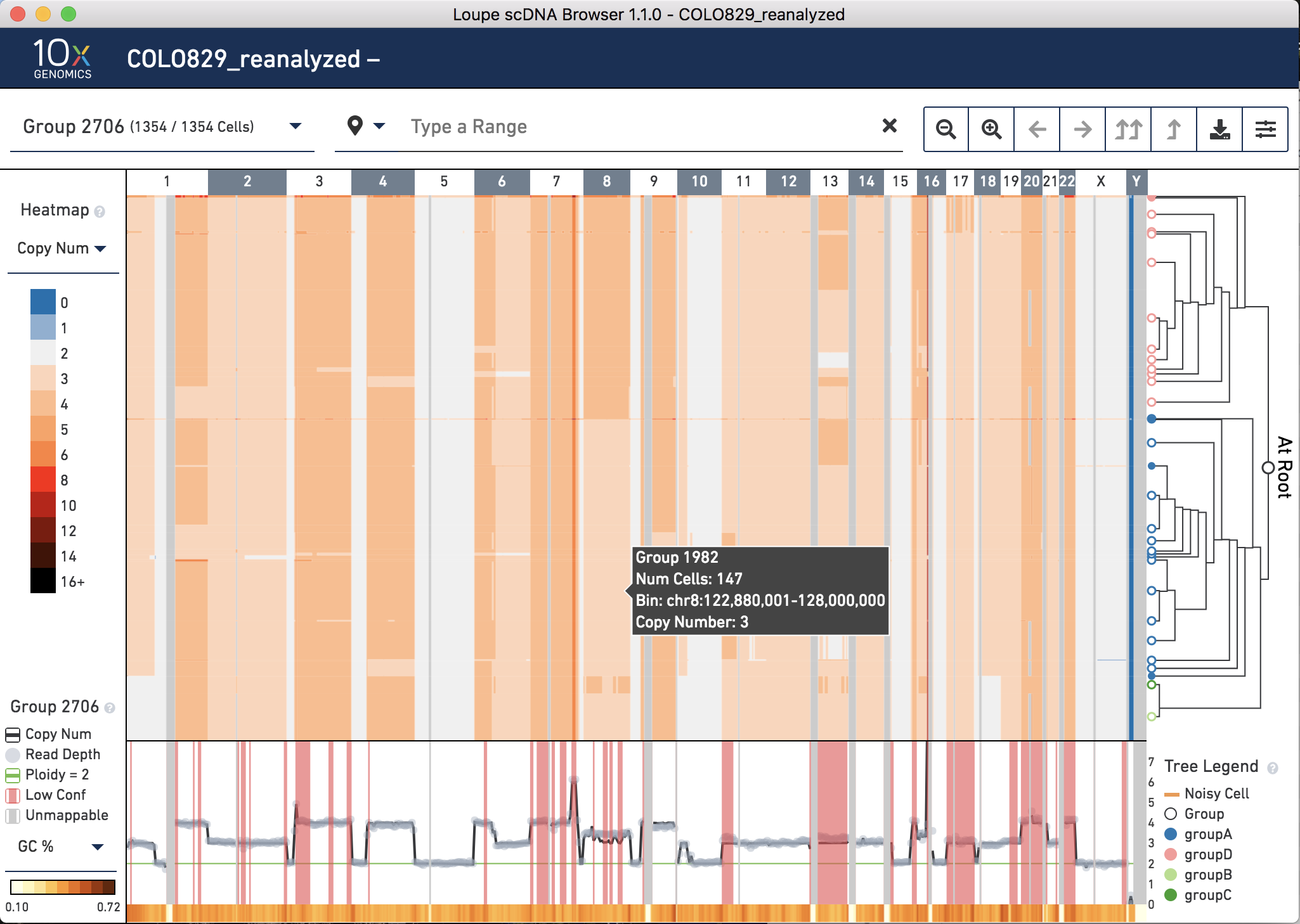
First, note that there are only 1,354 cells in the dataset now. The cells called as noisy in the original analysis have been removed. (Recall that a cell is classified as noisy if the ploidy_confidence from CNV calling is low or if the DIMAPD value is an outlier compared to the rest of the sample population). This can be seen on the top left next to Group 2706.
Second, notice on the bottom right in the tree legend, the four groups are annotated with different colors.
Third, note in the tree that group B is sister to group C, which combined (Group 1151) are sister to group A, with group D as the outgroup. Recall that this was specified by the newick file input, however, the relationships of cells within these groups is dictated by hierarchical clustering.
Now compare these groups to the events observed both in Figure 3 of Velazquez-Villarreal et al. (2019):
Are these events observed in the reanalyzed dloupe file? Start by clicking on Chromosome 1:
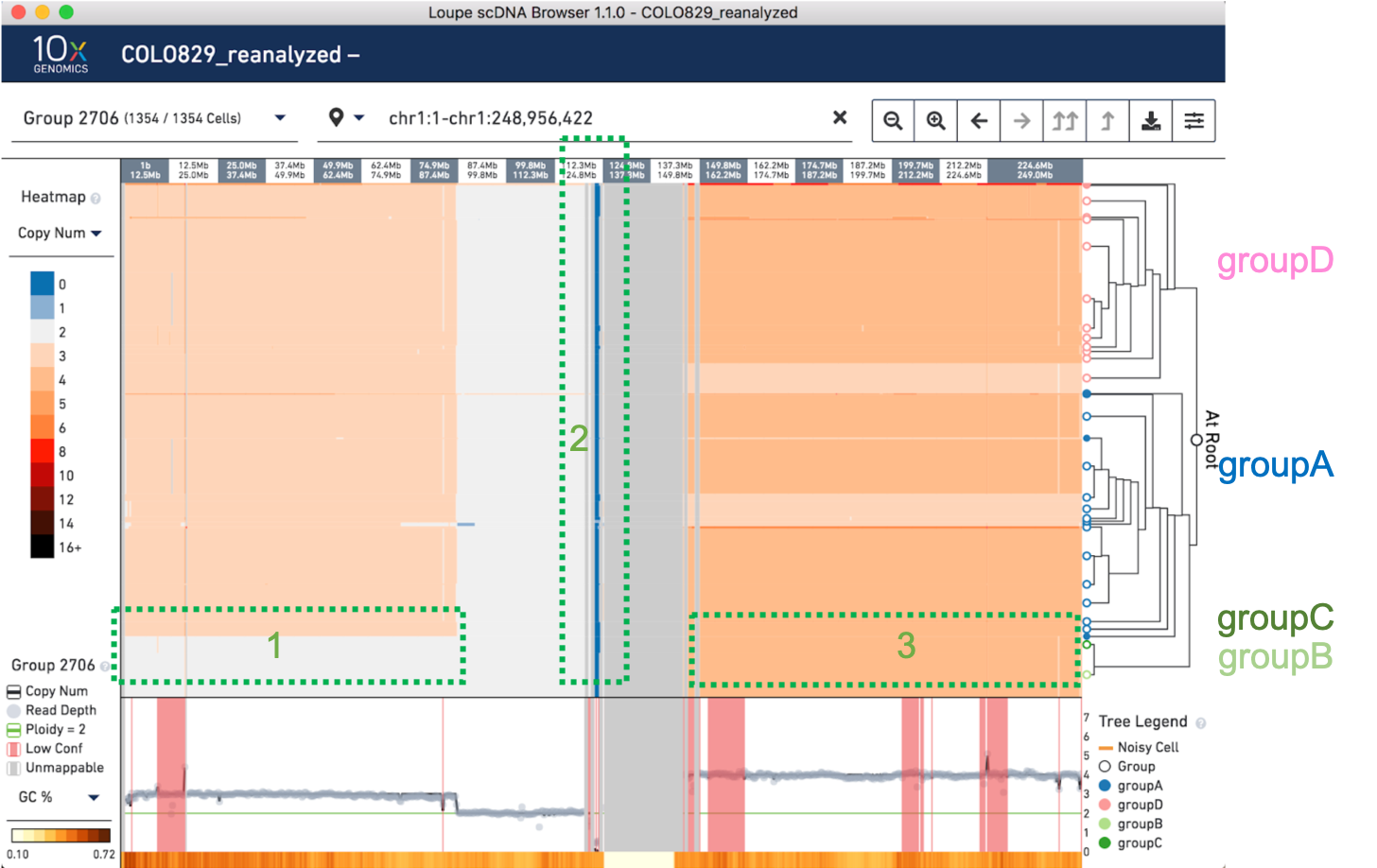
On the left side of the screen (highlighted in green as section 1) is the CNV that distinguishes groups A and D from B and C. There is also a large unmappable region in the center of the chromosome (highlighted in green as section 2) , likely a centromere. On the right side of the centromere (highlighted in green as section 3), there is some variation within the sample, but not the kind that separates the four major groups.
At this scale, we can see that there is a breakpoint in groups A and D where Chromosome 1 changes from copy number 3 to copy number 2, somewhere between 74.9 and 87.4 Mb. The breakpoint as reported by the manuscript is 1p22 (GRCh37 chr1:87,337,015). To zoom into the breakpoint, copy and paste chr1:85,700,001-chr1:87,500,000 into the top view to zoom in, or click and drag to manually zoom in.
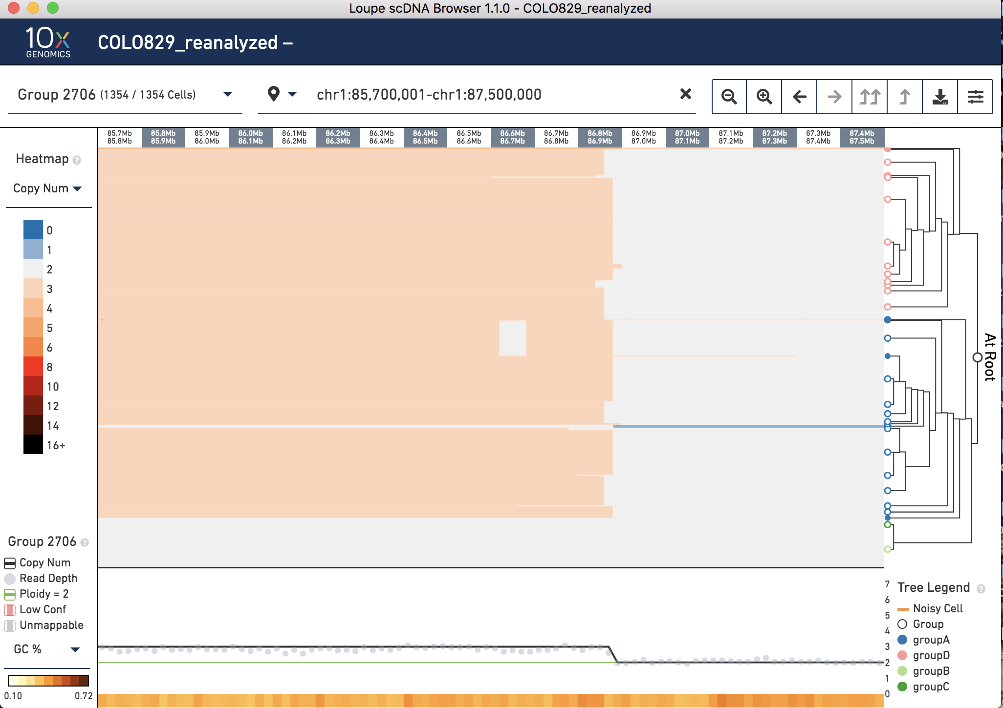
How well does it match up? In the .dloupe file with the GRCh38 reference it is called between 86.8 and 86.9 Mb in Groups A and D, with some variation between clusters, so about half a Mb off.
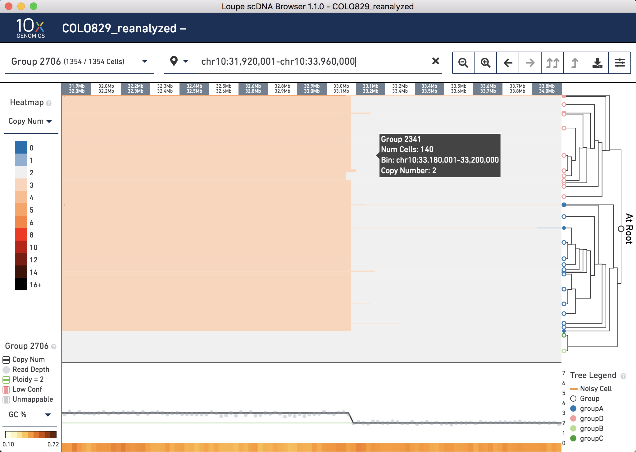
Click the X on the top navigation panel to zoom back out. Now do the same for Chromosome 10. Find the breakpoint 10p14 (GRCh37 chr10:36,119,061) which joins with the earlier identified breakpoint. Copy and paste chr10:31,920,001-chr10:33,960,000 into the top panel and note the breakpoint is called between 33.0 and 33.1 Mb:
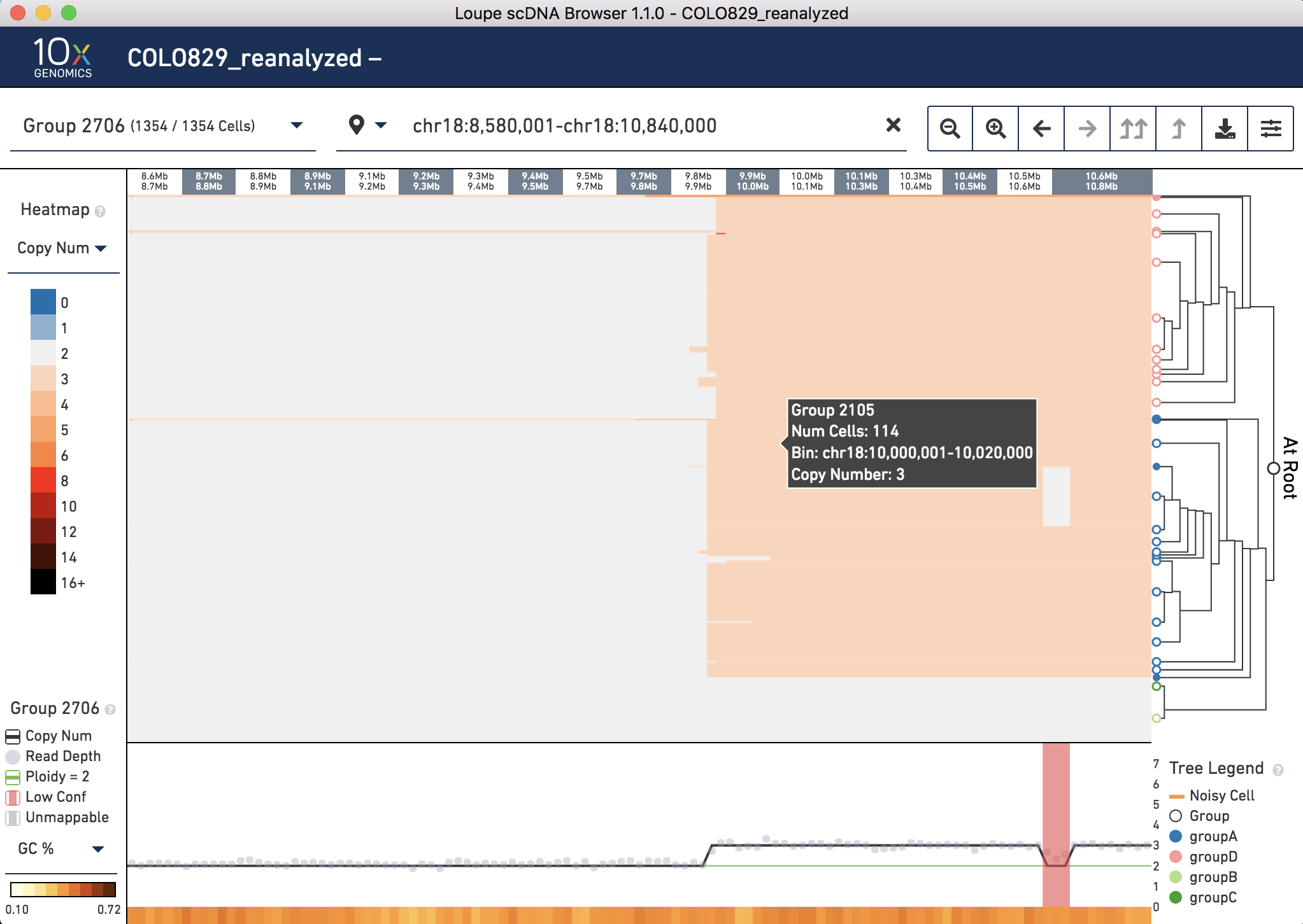
Finally, zoom in to Chromosome 18 (chr18:8,580,001-chr18:10,840,000), and note this CNV spans most of the chromosome on both sides of the unmappable centromere. Look for the breakpoint 18p11 (GRCh37chr18:9,868,810) which is where the 3' end of chr10 joins to. Here it is called between 9.8 and 9.9 Mb:
To review, we found support in the .dloupe file for several of the major CNV events described in the publication using third-party tools.
To perform a pseudo-bulk copy number and loss of heterozygosity analysis following Velazquez-Villarreal et al. (2019), reads across cells within a group must be combined before calling SNVs. The steps to demonstrate this are beyond the scope of this tutorial, but are covered in the paper. For SNV calling, 10x Genomics offers a fully supported pipeline, cellranger-dna bamslice, which subsets BAM files by cell barcodes. The split BAM files can be used as input for downstream analysis with third-party variant calling tools such as Mutect and GATK (not supported by 10x Genomics). The BAM files can also be converted to a FASTQ file format using the bamtofastq tool.
cellranger-dna bamslice uses the same input files used for cellranger-dna reanalyze. Set up a command as follows:
cellranger-dna bamslice --id=group_subsets \
--csv=/path/to/reanalyze_config.csv \
--bam=/path/to/outs/possorted_bam.bam \
--localmem=128 \
--localcores=16
You may wish to increase the amount of cores and memory, as this is a computationally intensive job that may take several hours. Ensure you have adequate disk space. If you used only one flowcell as described above, you will have 1.14 billion reads to slice, about 77 GB of disk space. For the purposes of the tutorial, there is no need to run the job to completion. If you do, you should observe four new bam files, one for each group as defined in the input CSV file.
Thus far, we have covered data generated from a single scCNV library that included cells that were run through a single Chromium chip channel, also known as a GEM Well. However, it can be advantageous to combine data from multiple libraries generated simultaneously or generated at different times previously. This can be particularly useful when comparing diseased vs. healthy samples, treatments vs. controls, multiple sections of a tissue, or different timepoints. Data from multiple libraries combined using cellranger dna aggr can be visualized in the Loupe scDNA browser.
One of the outputs of cellranger-dna aggr is a dloupe.dloupe file. To visualize an aggregated dataset, we use a public breast tumor tissue dataset that consists of five sections of approximately 2,000 cells each. By now, you should be familiar enough with the mechanics of running the Cell Ranger DNA pipeline, so we will skip this computationally intensive step. Download the dloupe file here and open it with Loupe scDNA Browser:
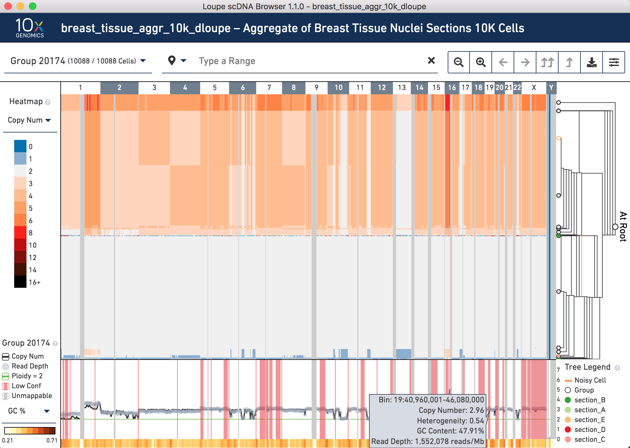
Notice there are 10,088 cells in these aggregated data. Broadly, the cells fall into two main categories – cells that are mostly diploid, and others that have regions of copy number gains.
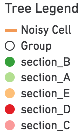
Note the legend on the bottom right shows which cells came from which section of the tumor:
Mouse over group 19603, in this case containing 152 cells, to see its relative composition from different cells across the tumor:
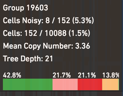
Click on this group to see more of the heterogeneity within it.
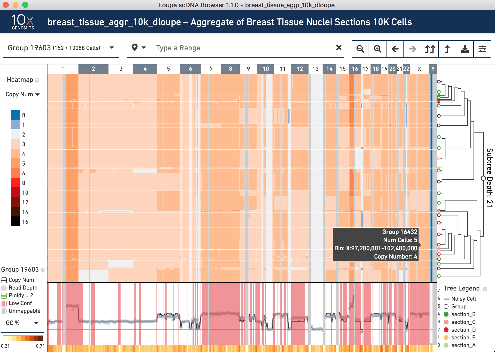
Change the heatmap on the left to Heterogeneity to see which of the clusters have higher or lower heterogeneity.
Congratulations, you have completed the tutorial. You now are able to complete the following objectives:
We value your feedback. Email any questions or concerns about this tutorial to support@10xgenomics.com.