Cell Ranger DNA1.0, printed on 04/02/2025
The observed coverage per cell for a fixed 20 kb genome bin is influenced by
These effects can be incorporated into a generative model where DNA in a fixed, unknown copy number state "emits" read pairs that are observed according to a Poisson distribution. The mean of the Poisson distribution is determined by the product of the copy number, the effect of GC content, the mappability, and the scale factor: Xi ∼ Poisson(S pi Q(gi) mi) where i is an index over all the mappable bins, X is the read coverage, S is the scale factor, p is the copy number, Q(g) is the impact of GC content g, and m the mappability.
We restrict the estimation of copy number to mappable 20 kb bins of the genome defined as bins with mappability greater than 90% as determined by the simulation procedure described earlier. These highly mappable bins comprise 85-90% of the human reference genome GRCh37 depending on the sequenced read length and insert size. After restricting ourselves to mappable bins we ignore the small modulation effect due to varying mappability.
To determine the effect of GC content we aggregate the read coverage across a window of consecutive mappable bins to minimize the effects of sampling noise at low depth. The aggregation window w is approximately the number of 20 kb bins that would have to be aggregated to reach a mean read count of 200 reads per window.
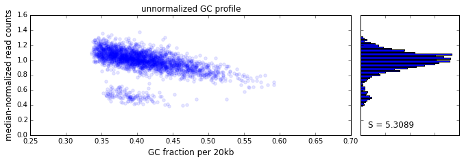
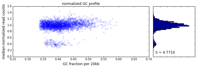
The effect of GC content on read coverage is made visually clear in the top panel of the plot above, where the read coverage (scaled to a mean of 1.0) is plotted against the GC content for a window size w = 20 (or 400 kb). The distinct bands are due to copy number variation in the cell: the lowest band corresponds to segments of copy number one, the next band to segments of copy number two, etc. The bottom panel shows the results after our GC correction procedure. The scaled GC-corrected coverage shows no relationship to the GC content.
We model the coverage variation as a multiplicative two parameter (l, q) quadratic function Q(g; l, q) of the GC content such that the variation is 1.0 at an arbitrarily chosen value GC = 0.45. When l and q are both zero this represents no variation of coverage with GC content. Given values of l, q we define the GC-corrected coverage y from the read coverage x yi=xiQ(gi;l,q) We find the best fit values of l, q by minimizing the entropy of the histogram of y.
We identify breakpoints in the read coverage that separate adjacent regions with distinct copy number by successive application of a log-likelihood ratio test based on the Poisson read-emission model described in the beginning of this page. Once all the breakpoints are identified the regions between two adjacent breakpoints define segments with uniform copy number.
For each mappable bin i in the genome and a half-open interval [l, r) around i we define the log-likelihood ratio (LLR) as LLR(i;l,r)=∑j∈[l,i)logProb(xj | μ[l,i))Prob(xj | μ[l,r))+∑j∈[i,r)logProb(xj | μ[i,r))Prob(xj | μ[l,r)) where μ[i,j)=∑i<=k<jxk∑i<=k<jQ(gk;l,q) The LLR helps decide between the hypotheses
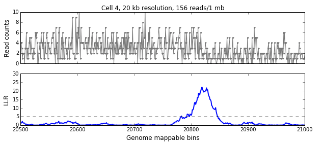
We calculate the LLR at each mappable bin i using a symmetric interval [i-w, i+w) around i, where w is the aggregation window defined in the previous section. The figure below shows the read-pair counts (x) for a single cell over 500 mappable bins (10 Mb) in the top panel and the calculated LLR for each bin in the bottom panel. The peak above the significance threshold of 5 indicates the presence of one or more breakpoints.
We use the following algorithm to identify breakpoints
We divide the genome into a set D of non-overlapping segments [l, r) based on the final breakpoint set where each segment is bounded by consecutive breakpoints l and r.
After segmentation we determine the integer copy number of each segment in D by estimating the scale factor S. We define an objective function defined as the length-weighted sum over all segments [l, r) O(S)=∑[l,r)∈D(r−l)sin2(πμ′[l,r)S) where μ′[l,r)=μ[l,r)w is the segment mean defined as the mean normalized read-pair count for each segment calculated over the aggregation window w. The objective function is minimized when each segment mean is an integer multiple of the scale factor S. The objective function has multiple local minima and each minimum defines a candidate copy number solution Ci=round(μ′[l,r)S) where [l, r) is the unique segment that contains the bin i. We filter out candidate solutions that are poor fits to the data or correspond to an average copy number greater than 8. We use the following heuristic to determine the best candidate copy number solution
For each region R with low mappability (simulated mappability < 0.90) we consider the copy number values of adjacent bins with high mappability determined. When the values agree and when R is less than 500 kb, we set the copy number across R equal to the copy number of the adjacent bins. When this is not the case, for example, in large centromeric regions, we designate R as a no call. See HDF5 Output for more information about how this imputation is conveyed in the outputs.
For every copy number n event in the interval [l, r) the generative Poisson model allows us to calculate a confidence score using the posterior distribution. For each bin i in the interval [l, r), we calculate the approximate posterior as
P(n)=Prob(xi | n)Prob(xi | n−1)+Prob(xi | n)+Prob(xi | n+1)
When we encounter Prob(x | 0) in the formula above, which occurs when n=0, 1, we substitute Prob(x | 0.01) instead since copy number 0 events do have non-zero read counts due to mis-mapped reads. We drop the Prob(x | n-1) term in the denominator when n=0.
P(n)=Prob(xi | n)Prob(xi | n−1)+Prob(xi | n)+Prob(xi | n+1)
We calculate the confidence score for the event using the bin-wise log-product
conf=−100(r−l)log10∏l≤i<r(1−P(n))
We multiply the score by 100 so we can truncate the confidence score to the interval [0, 256) and represent as uint8. When we have a good fit to the copy number n hypothesis, P(n) is very close to 1, and the confidence score is large and positive.