Cell Ranger ATAC1.1, printed on 02/01/2025
The computational pipeline for processing the data produced from the Chromium Single Cell ATAC Solution involves the following analysis steps:
This step is performed in order to fix the occasional sequencing error in barcodes so that fragments get associated with the original barcodes, thus improving data quality. The 16bp barcode sequence is obtained from the "I2" index read. Each barcode sequence is checked against a 'whitelist' of correct barcode sequences, and the frequency of each whitelist barcode is counted. We attempt to correct barcodes that aren't on the whitelist, by finding all whitelisted barcodes that are within 2 differences (Hamming distance <= 2) of the observed sequence, and scoring them based on the abundance of that barcode in the read data and quality value of the incorrect bases. An observed barcode not present in the whitelist is corrected to a whitelist barcode if it has > 90% probability of being the real barcode based on this model.
Cell Ranger ATAC performs reference-based analysis and requires adapter and primer oligo sequence to be trimmed off before mapping confidently. In the current chemistry, the 3' end of a read (the end of the read sequence) may contain the reverse complement of the primer sequence, if the read length is greater than the length of the genomic fragment. We use the cutadapt tool to identify the reverse complement of the primer sequence at the end of each read, and trim it from the read prior to alignment.
Then, the trimmed read-pairs are aligned to a specified reference using BWA-MEM with default parameters. Please note that BWA-MEM will not align reads less than 25bp. These unaligned reads are included in the BAM output and flagged as unmapped.
A barcoded fragment may get sequenced multiple times due to PCR amplification. We mark duplicates in order to identify the original fragments that constitute the library and contribute to its complexity. We find duplicate reads by identifying groups of read-pairs, across all barcodes, where the 5' ends of both R1 and R2 have identical mapping positions on the reference, correcting for soft-clipping. These groups of read-pairs arise from the same original molecule. Among these read-pairs, the most common barcode sequence is identified. One of the read-pairs with that barcode sequence is labelled the 'original' and the other read-pairs in the group are marked as duplicates of that fragment in the BAM file. If it passes the filters described in the next paragraph, this is the only read pair that is reported as a fragment in the fragment file, and it will be marked with the most-common barcode sequence.
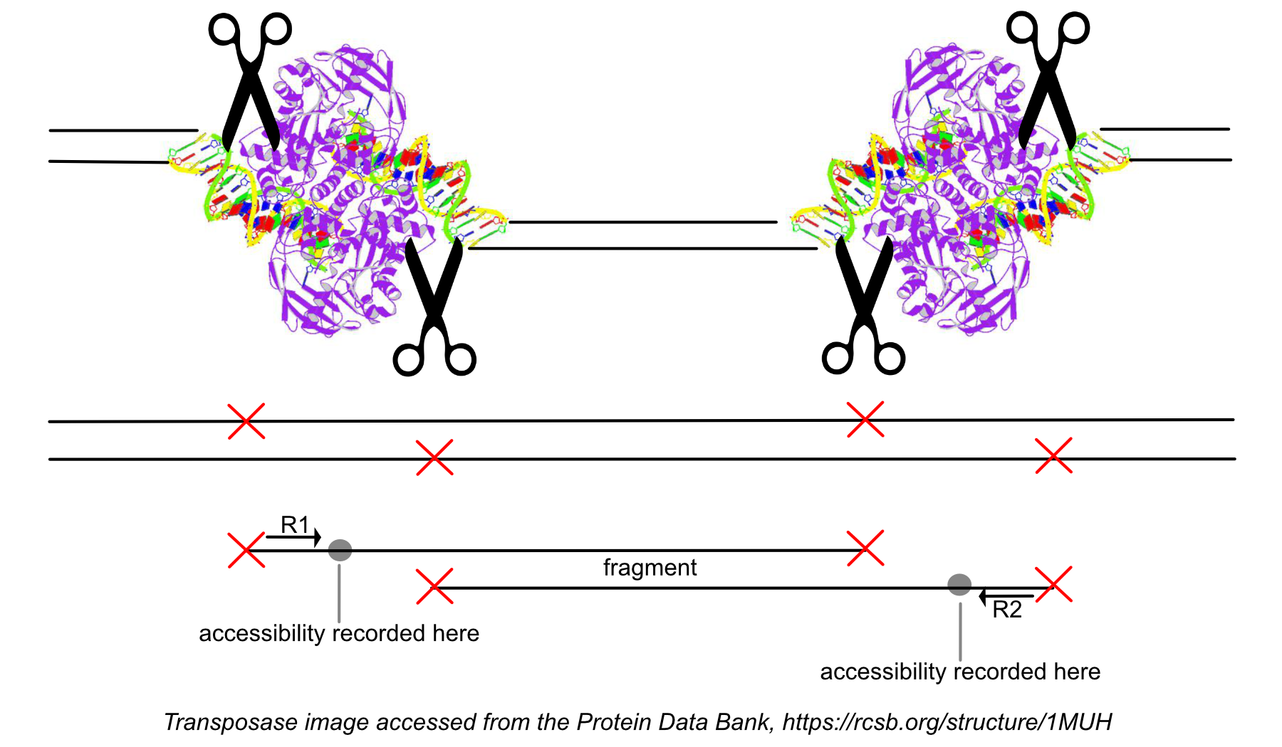
While processing the group of identically aligned read-pairs as described above, once the original fragment is marked, we determine if the fragment is mapped with MAPQ > 30 on both reads, is not mitochondrial, and not chimerically mapped. If the fragment passes these filters, we create one entry in the fragments.tsv.gz file marking the start and end of the fragment after adjusting the 5' ends of the read-pair to account for transposition, during which the transposase occupies a region of DNA 9 base pairs long (see figure). With this entry we associate the most common barcode observed for the group of read-pairs and the number of times this fragment is observed in the library (size of the group). Note that as a consequence of this approach, each unique interval on the genome can be associated with only one barcode. Each entry is tab-separated and the file is position-sorted and then run through the SAMtools tabix command with default parameters.
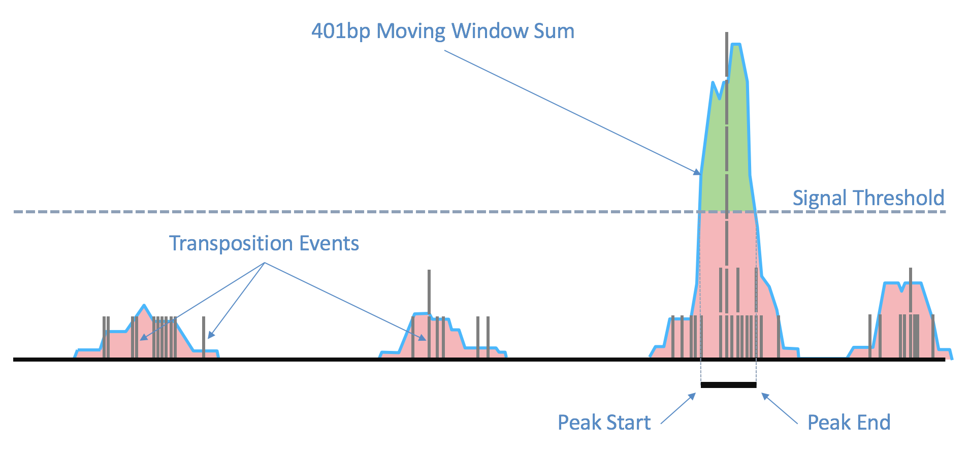
As the ends of each fragment are indicative of regions of open chromatin, we analyze the combined signal from these fragments to determine regions of the genome enriched for open chromatin and thus, putatively of regulatory and functional significance. Using the sites as determined by the ends of the fragments in the position-sorted fragments.tsv.gz file, we count the number of transposition events at each base-pair along the genome. We generate a smoothed profile of these events with a 401bp moving window sum around each base-pair and fit a ZINBA-like mixture model consisting of geometric distribution to model zero-inflated count, negative binomial distribution to model noise and another geometric distribution to model the signal. We set a signal threshold based on an odds-ratio of 1/5 that determines, at base pair resolution, whether a region is a peak signal (enriched for open chromatin) or noise. Consequently, not all cut sites are within a peak region. Peaks within 500bp of each other are merged to produce a position-sorted BED file of peaks. The window size, the odds-ratio and the distance to merge peaks were selected to maximize the area under the receiver-operator curve when the peaks are compared to a high-quality list of DNase hypersensitive sites for GM12878 from ENCODE, and also to produce satisfactory clustering metrics as well as cell type identification in a set of peripheral blood mononuclear cells (PBMC) libraries. This method of identifying peaks is independent of barcodes and their cellular (or non-cell) identity, which allows us to include the signal from all real genomic fragments as determined by mapping. A theoretical disadvantage of such a method would be not being able to identify rare peaks appearing only in very rare populations.
This step associates a subset of barcodes observed in the library to the cells loaded from the sample. Identification of these cell barcodes allows one to then analyze the variation in data at single cell resolution. For each barcode, we have the record of mapped high-quality fragments that passed all filters (the fragments.tsv file). Having determined peaks prior to this, we use the number of fragments that overlap any peak regions, for each barcode, to separate the signal from noise. This works better in practice as compared to naively using the number of fragments per barcode. The cell calling is done in two steps. First we identify barcodes that have fraction of fragments overlapping called peaks lower than the fraction of genome in peaks (for the sake of this calculation only, peaks are padded by 2000 bp on both sides to account for fragment length). We have found that these barcodes typically have their cut sites randomly distributed over the genome, are not targeted to be enriched near functional regions, and do not exhibit the expected ATAC-seq "peaky" signal. Therefore we mask these barcodes out of the total set of barcodes observed for the library, and perform cell calling on the remainder barcodes. We subtract a depth-dependent fixed count from all barcode counts to model whitelist contamination. This fixed count is the estimated number of fragments per barcode that originated from a different GEM, assuming a contamination rate of 0.02. Then we fit a mixture model of two negative binomial distributions to capture the signal and noise. Setting an odds ratio of 100000 (which appeared to work best with internal testing), we separate the barcodes that correspond to real cells from the non-cell barcodes.
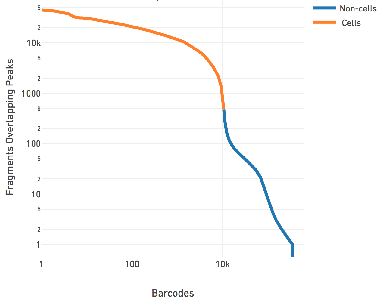
The cell calling is limited to produce < 20k cells per species in the reference as the assay is currently designed to support 500-10k cells. If --force-cells=N is provided as a parameter to Cell Ranger ATAC, we ensure that the top N barcodes are reported as cells for each species, as per the barcode rank plot above. N > 20k will not be accepted by the pipeline. If --force-cells is not provided, in the case of mixed species sample, we do a second iteration where we mask out the non-cell barcodes and fit the same mixture model to the two species distributions present in the cell barcodes and refine the division of cell barcodes associated with each species. In general, the --force-cells value to be used should correspond to a point below the "knee" as seen on the barcode rank plot above.
Similar to our analysis pipelines for the Single Cell Gene Expression Solution and the Single Cell Immune Profiling Solution, we produce a count matrix consisting of the counts of fragment ends (or cut sites) within each peak region for each barcode. This is the raw peak-barcode matrix and it captures the enrichment of open chromatin per barcode. The matrix is then filtered to consist of only cell barcodes, which is then used in subsequent analysis such as dimensionality reduction, clustering and visualization.
Biological discovery is often aided by visualization tools that allow one to group and compare a population of cells with another. In order to enable discovery, Cell Ranger ATAC performs clustering and t-SNE projection. As the data is sparse at single cell resolution, we first perform dimensionality reduction to cast it into a lower dimensional space, which also has the benefit of de-noising. Cell Ranger ATAC supports dimensionality reduction via Principal Component Analysis (PCA), Latent Semantic Analysis (LSA), or Probabilistic Latent Semantic Analysis (PLSA). The adopted default method is LSA, but users can specify which method to use by providing the dimensionality reduction parameter (--dim-reduce=<Method>) to Cell Ranger ATAC. Each of these methods acts on the filtered peak-barcode matrix consisting of cut site counts for cell barcodes in called peaks. Each method has an associated data normalization technique used prior to dimensionality reduction and a collection of clustering methods that accept the data after dimensionality reduction. We also provide an optimized implementation of the Barnes Hut TSNE algorithm (which is the same as the one in our analysis pipeline for the Single Cell Gene Expression Solution). The number of dimensions is fixed to 15 as it was found to sufficiently separate clusters visually and in a biologically meaningful way when tested on peripheral blood mononuclear cells (PBMCs).
For PCA, we first normalize the data to median cut site counts per barcode and log-transform it. We use a fast, scalable and memory efficient implementation of IRLBA (Augmented, Implicitly Restarted Lanczos Bidiagonalization Algorithm) that allows in-place centering and feature scaling and produces the transformed matrix along with the principal components (PC) and singular values encoding the variance explained by each PC. Specific to PCA, we provide k-means clustering that produces 2 to 10 clusters for visualization and analysis. We also provide a k-nearest neighbors graph-based clustering method via community detection using louvain modularity optimization algorithm. The transformed matrix is operated on by the t-SNE algorithm with default parameters and provides 2-D coordinates for each barcode for visualization. Users experienced with our Single Cell Gene Expression Solution may recognize that the analysis performed using PCA is akin to running Cell Ranger (cellranger count).
Inspired by the large body of work in the field of information retrieval, we normalize the data via the inverse-document frequency (idf) transform where each peak count is scaled by the log of the ratio of the number of barcodes in the matrix and the number of barcodes where the peak has a non-zero count. This provides greater weight to counts in peaks that occur in fewer barcodes. Singular value decomposition (SVD) is performed on this normalized matrix using IRLBA without scaling or centering, to produce the transformed matrix in lower dimensional space, as well as the components and the singular values signifying the importance of each component. Prior to clustering, we perform normalization to depth by scaling each barcode data point to unit L2-norm in the lower dimensional space. We found that the combination of these normalization techniques obviates the need to remove the first component. Specific to LSA, we provide spherical k-means clustering that produces 2 to 10 clusters for downstream analysis. Spherical k-means was found to perform better than plain k-means, by identifying clusters via k-means on L2-normalized data that lives on the spherical manifold. Similar to PCA, we also provide a graph-based clustering and visualization via t-SNE. However, similar to spherical k-means clustering, we normalize the data to unit norm before performing graph-based clustering and t-SNE projection.
PLSA is a special type of non-negative matrix factorization, with roots in Natural Language Processing. In PLSA we minimize, via an Expectation-Maximization algorithm, the KL-divergence between the empirically determined probability of observing a peak in a barcode and the lower rank approximation to it. We do not normalize the data prior to dimensionality reduction via PLSA. Similar to LSA and PCA, we produce a transformed matrix, component vectors and a set of values explaining the importance of each component. PLSA offers natural interpretation of the components and the transformed matrix. Each component could be interpreted as a hidden topic and the transformed matrix is simply the probability of observing a barcode from a given topic, i.e. Prob(barcode|topic). The component vectors are the probability of observing a peak from a given topic (Prob(peak|topic)) and the counterpart to singular values of LSA/PCA are simply the probability of each topic (Prob(topic)) observed in the data. Similar to LSA, we normalize the transformed matrix to unit L2-norm and perform spherical k-means clustering to produce 2 to 10 clusters, as well as graph-based clustering and visualization via t-SNE. While PLSA offers great advantages in interpretability of the lower dimensional space, it is appreciably slower than both PCA and LSA and does not scale well beyond 20 components on large datasets. To ameliorate this to some extent, the in-house implementation of PLSA is multithreaded (4 threads on compute cluster) and written and compiled in C++. To ensure a reasonable run time, the algorithm is capped at 3000 iterations if it doesn't converge first.
Below is the summary of dimensionality reduction techniques and associated clustering and visualization approaches provided in the pipeline.
| Dimensionality Reduction | Clustering | Visualization |
|---|---|---|
| PCA | K-means, graph-clustering | TSNE |
| LSA | Spherical k-means, graph-clustering | TSNE |
| PLSA | Spherical k-means, graph-clustering | TSNE |
| Note that in version 1.0 of the Cell Ranger ATAC pipelines, we provided k-medoids clustering. Spherical k-means was found to be an effective replacement for k-medoids for both LSA and PLSA, with a significant performance gain that makes it suitable to cluster large scale datasets you can expect from aggregation runs. |
As peaks are regions enriched for open chromatin, and thus have potential for regulatory function, observing the location of peaks with respect to genes can be insightful. We use bedtools closest -D=b to associate each peak with genes based on closest transcription start sites (packaged within the reference) such that the peak is within 1000 bases upstream or 100 bases downstream of the TSS. Additionally, we also associate genes to putative distal peaks that are much further from the TSS, and are less than 100kb upstream or downstream from the ends of the transcript. This association is adopted by our companion visualization software (Loupe Cell Browser) and used to construct and visualize derived features such as promoter-sums that pool together counts from peaks associated with a gene. Peaks are enriched for transcription factor (TF) binding motifs and the presence of certain motifs can be indicative of transcription factor activity. To identify these motifs, we first calculate the GC% distribution of peaks and then bin the peaks into equal quantile ranges in the GC content distribution. We use the MOODS Python library packaged inside Cell Ranger ATAC to scan each peak for matches to motif position-weight-matrices (PWMs) for transcription factors from the JASPAR database built directly into the reference package. We set a p-value threshold of 1E-7 and background nucleotide frequencies to be the observed nucleotide frequencies within the peak regions in each GC bucket. The list of motif-peak matches is unified across these buckets, thus avoiding GC bias in scanning.
As transcription factors (TF) tend to bind at sites containing their cognate motifs, grouping of accessibility measurements at peaks with common motifs produces a useful enrichment analysis of TFs across single cells. We construct an integer count for each TF for each cell barcode in the following manner: we consider all peaks matched to a given TF, as discovered in the TF motif detection. Then for every barcode, we pool together the cut-site counts across these matched peaks in the filtered peak-barcode matrix. This calculates the total cut-sites in a cell barcode for peaks that share the TF motif. We calculate the proportion of cut-sites for a TF within a barcode out of the total cut-sites for that barcode, which normalizes it to depth. We detect enrichment for a TF by z-scoring the distribution over barcodes of these proportion values for given TF. To make it robust to outliers, we use the modified z-score calculated using the median and the scaled median absolute deviation from the median (MAD), instead of the mean and standard deviation. These z-scored values are visible when you load a dataset in Loupe and accompanies the differential analysis built into Loupe Cell Browser.
| We do not produce the tf-barcode matrix for multi-species experiments or if the motifs.pfm file is missing from the reference package (for example in custom references). We cannot perform TF motif enrichment analysis in these cases. |
In order to identify transcription factor motifs whose accessibility is specific to each cluster, Cell Ranger ATAC tests, for each motif and each cluster, whether the in-cluster mean differs from the out-of-cluster mean. Users familiar with our Single Cell Gene Expression Solution may recognize that this is identical to what Cell Ranger does for identifying differential gene expression. In order to find differentially accessible motifs between groups of cells, Cell Ranger ATAC uses a Negative Binomial (NB2) generalized linear model to discover the cluster specific means and their standard deviations, and then employs a Wald test for inference. For each cluster, the algorithm is run on that cluster versus all other cells, yielding a list of TF motifs that are differentially expressed in that cluster relative to the rest of the sample. Using a GLM framework allows us to model the sequencing depth per cell and GC content in peaks per cell directly as covariates. This allows us to normalize to them naturally as part of model estimation and inference procedure. We also perform differential enrichment analysis for accessibility in peaks using a Poisson generalized linear model, much the same way as we do for TF motifs. In this case, we model only the per cell depth as a covariate.
| We cannot perform differential analysis for transcription factor motifs in the cases where the motifs.pfm file is missing from the reference package, such as in custom references built without the motif file or in multi-species experiments. We will always perform differential analysis on accessibility in peaks for single species references. |
In the aggr pipeline, user can provide a list of libraries to aggregate. The aggregation pipeline performs the task of merging the fragments from each listed library into one aggregated file, based on the normalization mode specified at runtime. The merger is performed by downsampling each library, with rates determined by the normalization mode. If the normalization mode is "None", all the fragments are retained and merged together. If the normalization mode is "depth", then each library is downsampled to have the same sensitivity (defined as per cell median number of fragments). If the normalization mode is "signal", the downsampling rates are determined using the information from the distribution of cut sites along the genome for each library. Specifically, for each library, a distribution of windowed cut sites counts is constructed and the 3-component mixture model is fit, identical to what we do in peak calling. The downsampling rates are set by matching the mean of the signal component for each library. Once the fragments are merged together, they are sorted by position and tabixed for downstream use such as dimensionality reduction, clustering, visualization and differential analysis.